Chapter 2 Added variable plots

p. 54 Figure 3.3(a)

Compute the regression of lifeExpF on log(ppgdp):

library(alr4)
library(tidyverse)
library(plotly)
u <- UN11

mod1 <- lm(u$lifeExpF ~ log(u$ppgdp))
mod1

## 
## Call:
## lm(formula = u$lifeExpF ~ log(u$ppgdp))
## 
## Coefficients:
##  (Intercept)  log(u$ppgdp)  
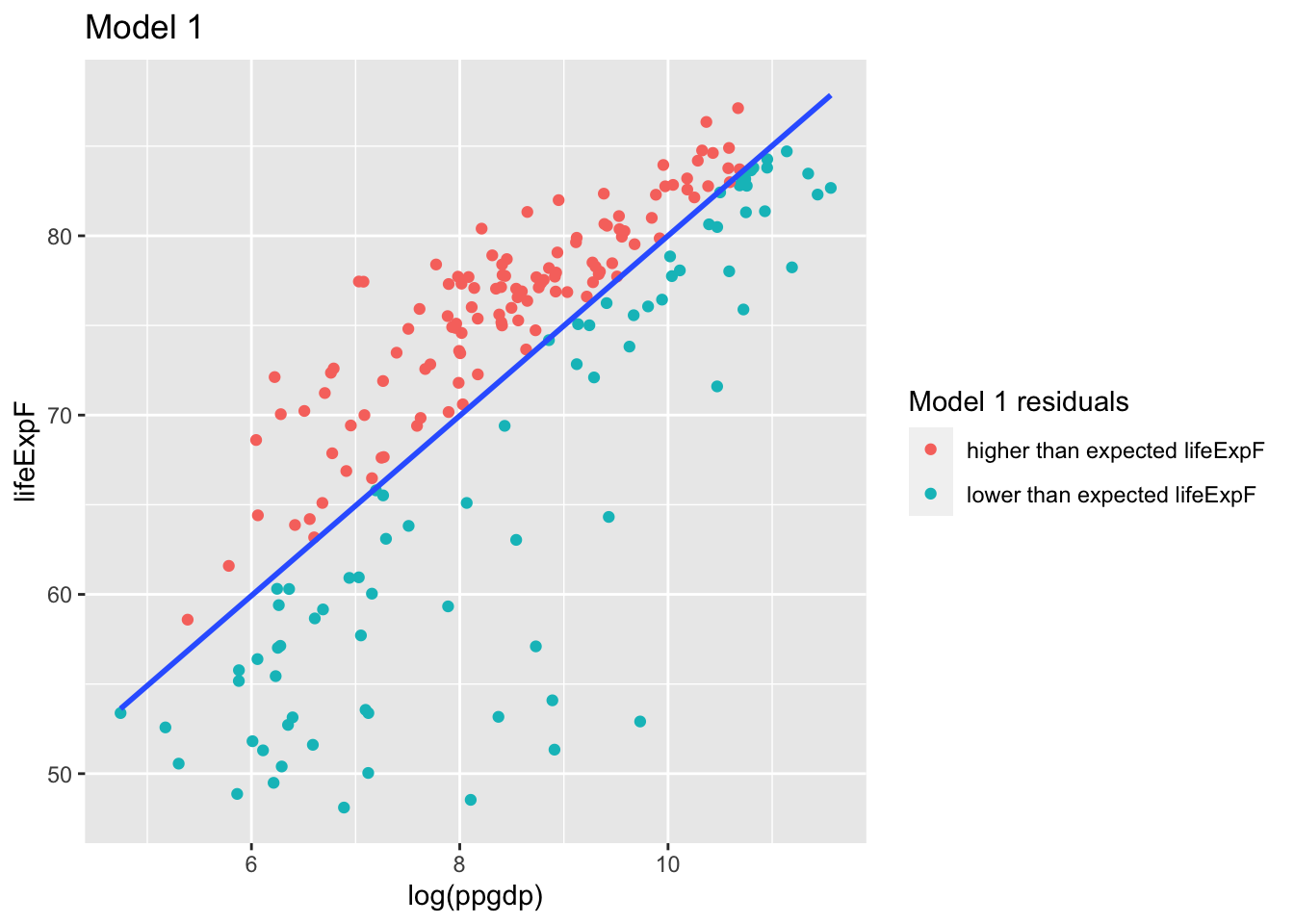
##       29.815         5.019

summary(mod1)$r.squared

## [1] 0.5963835

u$`Model 1 residuals` <- ifelse(mod1$residuals > 0, "higher than expected lifeExpF", "lower than expected lifeExpF")

g <- ggplot(u, aes(log(ppgdp), lifeExpF, label = rownames(u), color = `Model 1 residuals`)) + 
  geom_point() +  
  geom_smooth(aes(group = 1), method = "lm", se=FALSE, show.legend =FALSE) +
  ggtitle("Model 1")
g

The residuals from this model are the part of the response lifeExpF not explained by the regression on log(ppgdp)

Compute the regression of fertility on log(ppgdp).

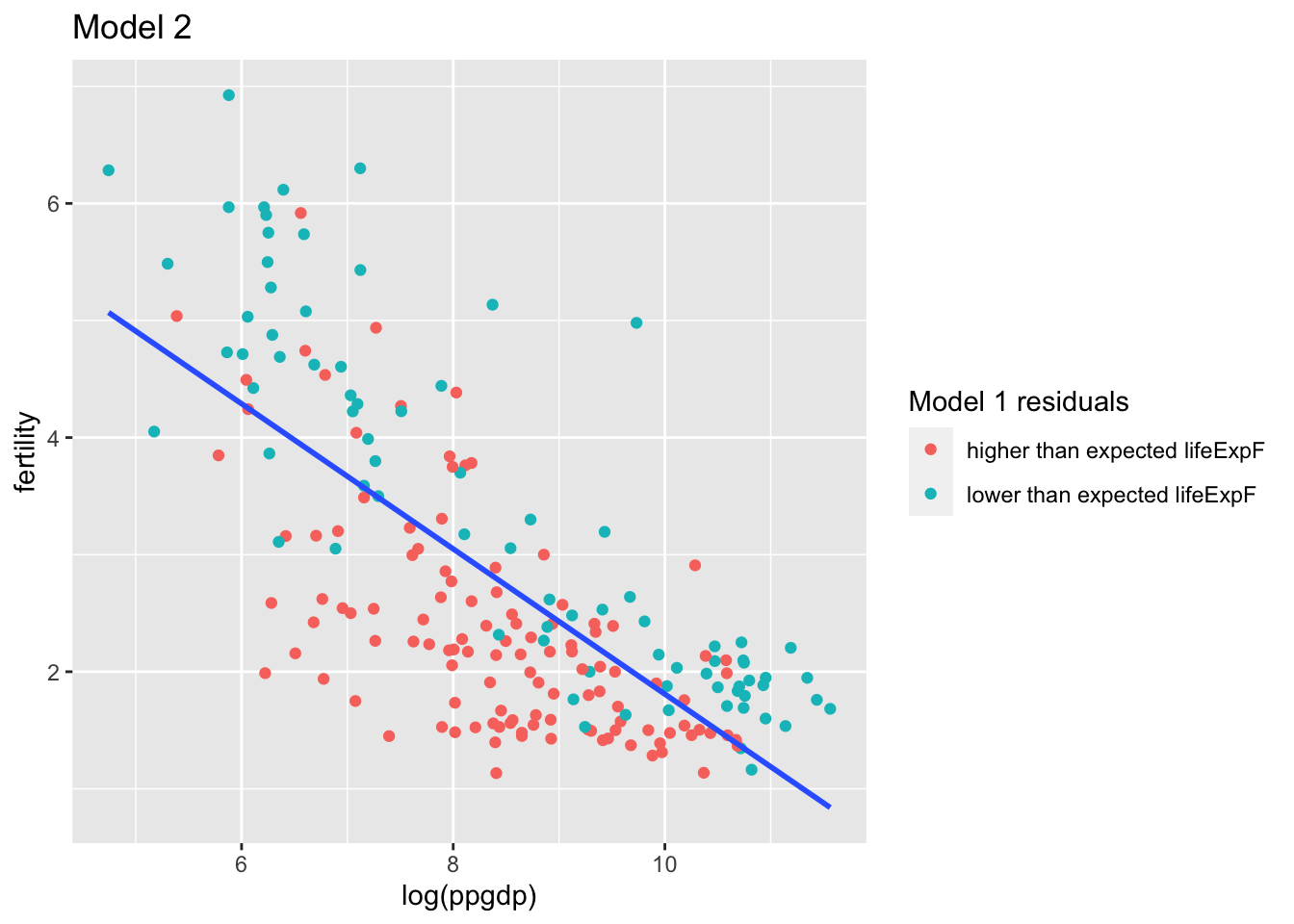
The residuals from this model are the part of the new regressor fertility not explained by the regression on log(ppgdp)

mod2 <- lm(u$fertility ~ log(u$ppgdp))
mod2

## 
## Call:
## lm(formula = u$fertility ~ log(u$ppgdp))
## 
## Coefficients:
##  (Intercept)  log(u$ppgdp)  
##       8.0097       -0.6201

summary(mod2)$r.squared

## [1] 0.5199563

g <- ggplot(u, aes(log(ppgdp), fertility, label = rownames(u), color = `Model 1 residuals`)) + 
  geom_point() +
  geom_smooth(aes(group = 1), method = "lm", se=FALSE, show.legend = FALSE) +
  ggtitle("Model 2")
g

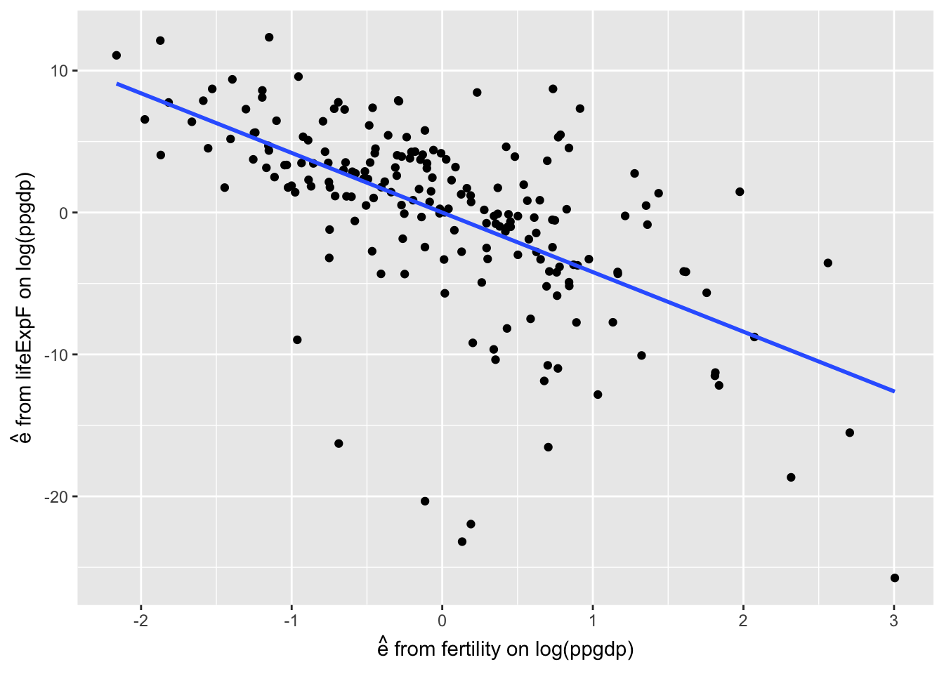
The added variable plot is of the unexplained part of the response from (1) on the unexplained part of the added regressor from (2).

residdf <- tibble::tibble(r1 = mod1$residuals,
                          r2 = mod2$residuals)
g <- ggplot(residdf, aes(r2, r1)) + 
  geom_point() +
  xlab(expression(paste(hat(e), " from fertility on log(ppgdp)"))) +
  ylab(expression(paste(hat(e), " from lifeExpF on log(ppgdp)"))) +
  geom_smooth(method = "lm", se=FALSE)
g

The slope of this regression line is:

lm(residdf$r1~residdf$r2)

## 
## Call:
## lm(formula = residdf$r1 ~ residdf$r2)
## 
## Coefficients:
## (Intercept)   residdf$r2  
##   7.681e-16   -4.199e+00

It is the same as the coefficient of \(\hat{\beta_2}\) with both regressors:

u$logppgdp <- log(u$ppgdp)
mod <- lm(lifeExpF ~ fertility + logppgdp, data = u)
mod

## 
## Call:
## lm(formula = lifeExpF ~ fertility + logppgdp, data = u)
## 
## Coefficients:
## (Intercept)    fertility     logppgdp  
##      63.448       -4.199        2.415