4  Jade Chapter

library(tidyverse)
df <- read_csv("https://data.cityofnewyork.us/resource/uip8-fykc.csv")
str(df)

spc_tbl_ [1,000 × 19] (S3: spec_tbl_df/tbl_df/tbl/data.frame)
 $ arrest_key       : num [1:1000] 3.18e+08 3.18e+08 3.19e+08 3.19e+08 3.19e+08 ...
 $ arrest_date      : POSIXct[1:1000], format: "2026-01-06" "2026-01-03" ...
 $ pd_cd            : num [1:1000] 105 203 105 397 397 263 548 777 109 397 ...
 $ pd_desc          : chr [1:1000] "STRANGULATION 1ST" "TRESPASS 3, CRIMINAL" "STRANGULATION 1ST" "ROBBERY,OPEN AREA UNCLASSIFIED" ...
 $ ky_cd            : num [1:1000] 106 352 106 105 105 114 350 NA 106 105 ...
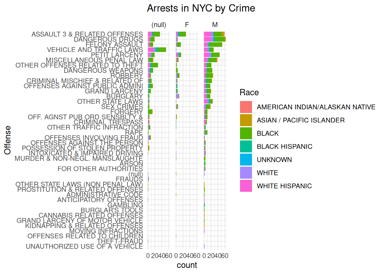
 $ ofns_desc        : chr [1:1000] "FELONY ASSAULT" "CRIMINAL TRESPASS" "FELONY ASSAULT" "ROBBERY" ...
 $ law_code         : chr [1:1000] "PL 1211200" "PL 140100G" "PL 1211200" "PL 160102B" ...
 $ law_cat_cd       : chr [1:1000] "F" "M" "F" "F" ...
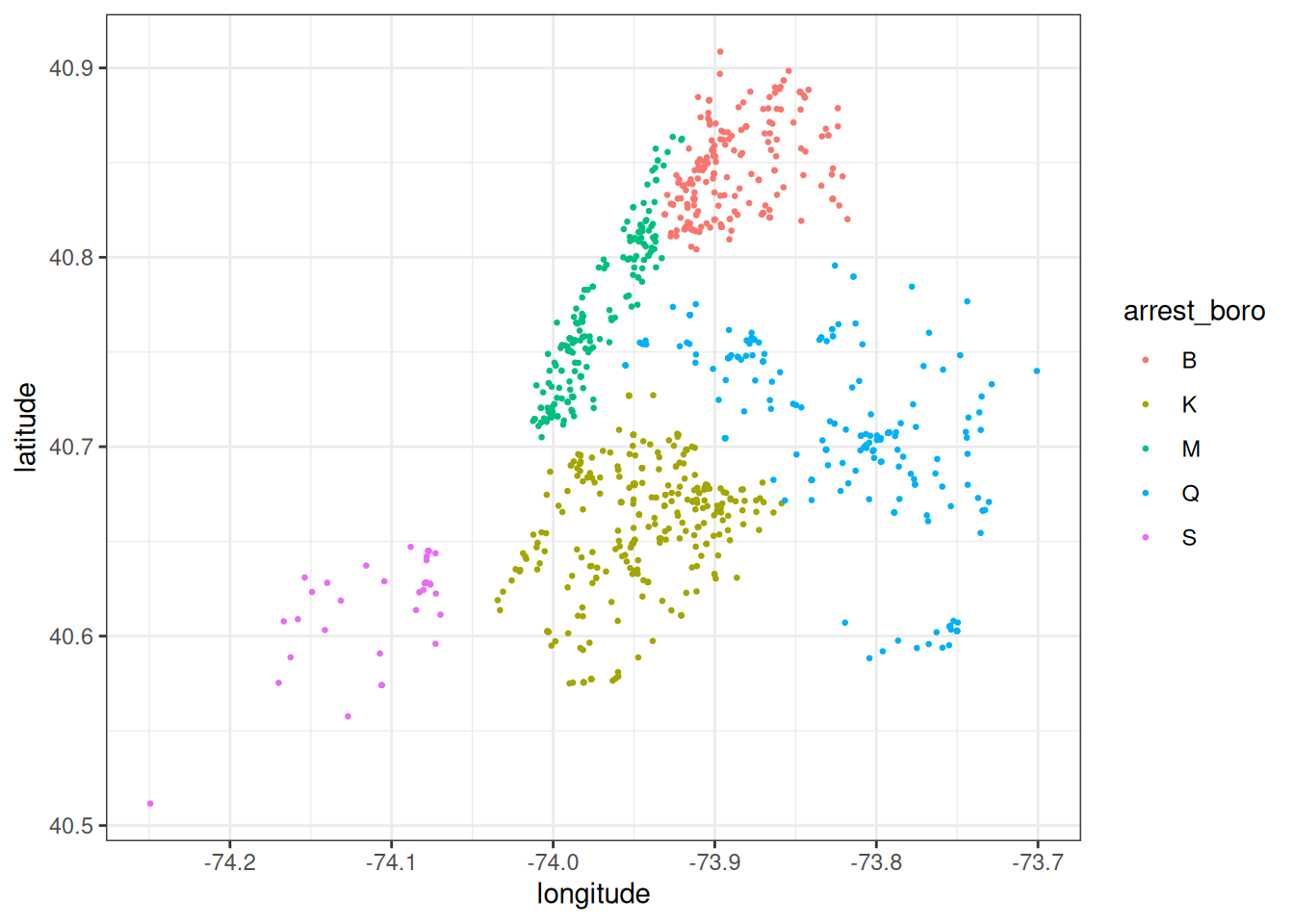
 $ arrest_boro      : chr [1:1000] "Q" "K" "B" "M" ...
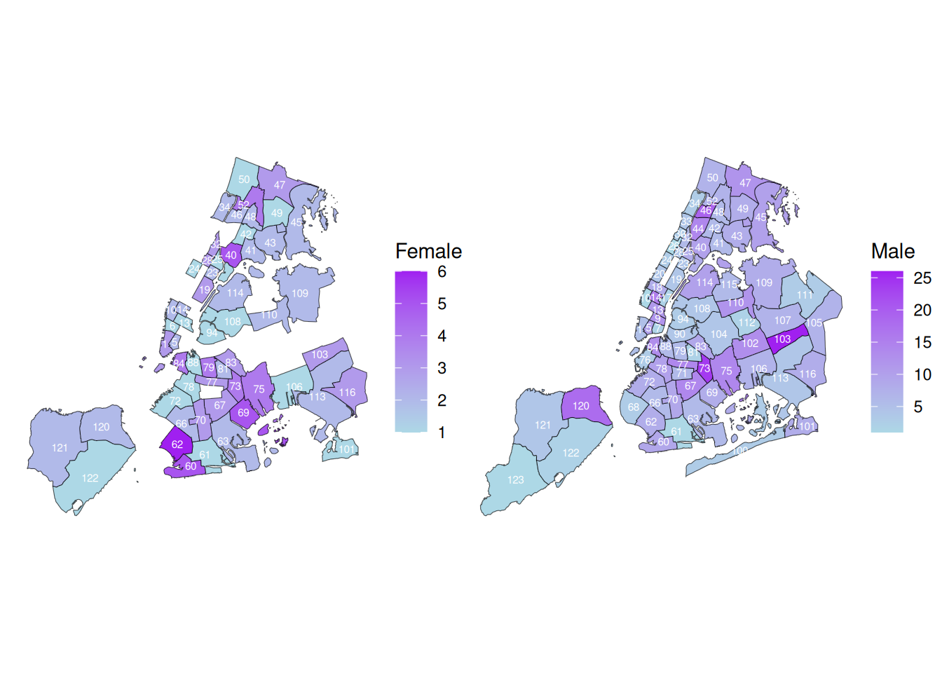
 $ arrest_precinct  : num [1:1000] 110 77 48 28 45 28 41 67 120 103 ...
 $ jurisdiction_code: num [1:1000] 0 1 0 0 0 0 0 0 0 0 ...
 $ age_group        : chr [1:1000] "25-44" "25-44" "25-44" "(null)" ...
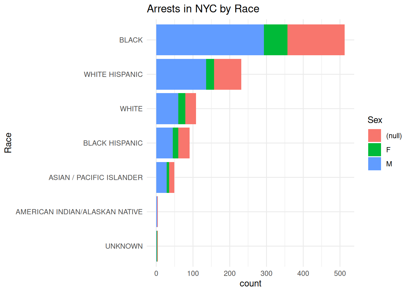
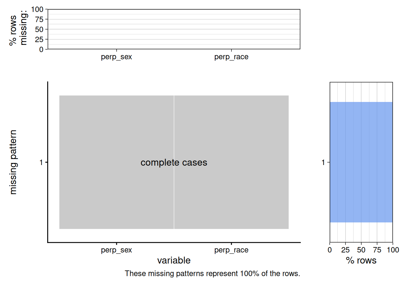
 $ perp_sex         : chr [1:1000] "M" "M" "M" "(null)" ...
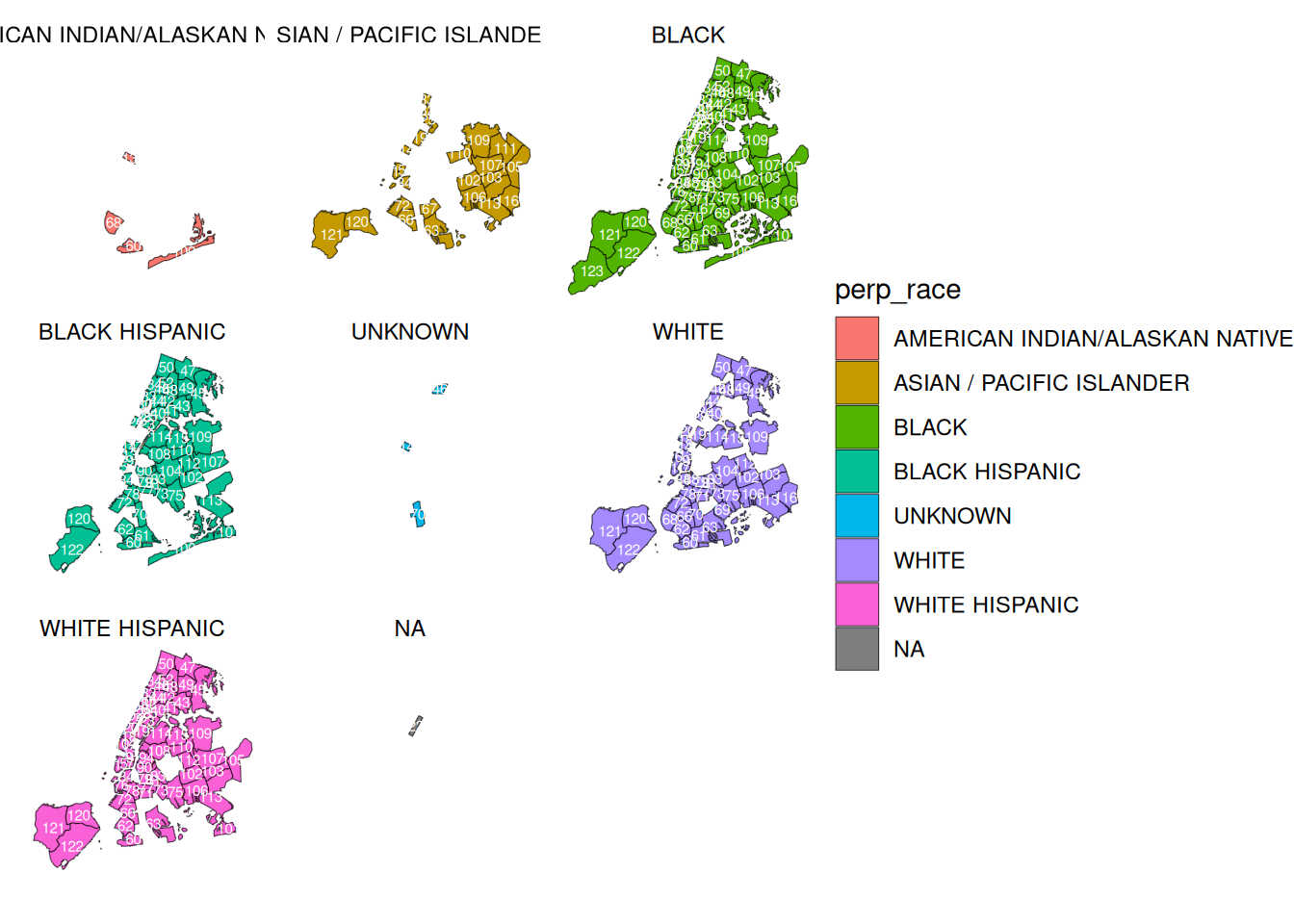
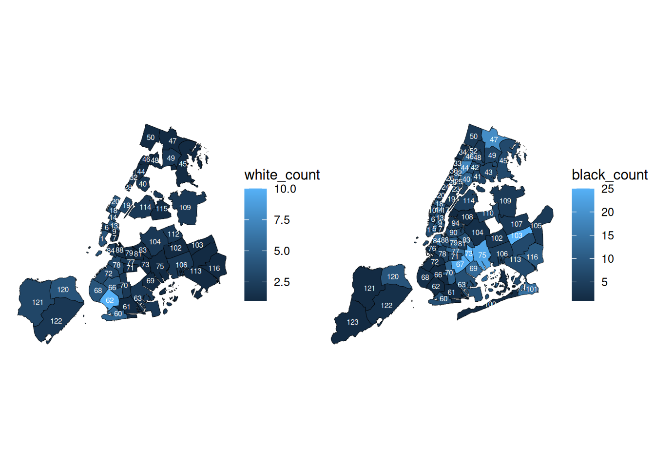
 $ perp_race        : chr [1:1000] "BLACK" "BLACK" "WHITE HISPANIC" "BLACK" ...
 $ x_coord_cd       : num [1:1000] 1020232 1003358 1011780 999788 1031351 ...
 $ y_coord_cd       : num [1:1000] 210719 182945 246837 233328 254245 ...
 $ latitude         : num [1:1000] 40.7 40.7 40.8 40.8 40.9 ...
 $ longitude        : num [1:1000] -73.9 -73.9 -73.9 -73.9 -73.8 ...
 $ geocoded_column  : chr [1:1000] "POINT (-73.870145 40.744989)" "POINT (-73.93112014 40.66879784)" "POINT (-73.9005 40.844152)" "POINT (-73.943874 40.807102)" ...
 - attr(*, "spec")=
  .. cols(
  ..   arrest_key = col_double(),
  ..   arrest_date = col_datetime(format = ""),
  ..   pd_cd = col_double(),
  ..   pd_desc = col_character(),
  ..   ky_cd = col_double(),
  ..   ofns_desc = col_character(),
  ..   law_code = col_character(),
  ..   law_cat_cd = col_character(),
  ..   arrest_boro = col_character(),
  ..   arrest_precinct = col_double(),
  ..   jurisdiction_code = col_double(),
  ..   age_group = col_character(),
  ..   perp_sex = col_character(),
  ..   perp_race = col_character(),
  ..   x_coord_cd = col_double(),
  ..   y_coord_cd = col_double(),
  ..   latitude = col_double(),
  ..   longitude = col_double(),
  ..   geocoded_column = col_character()
  .. )
 - attr(*, "problems")=<pointer: 0x5623ae6ad560> 

df <- df |>
  rename(Precinct = arrest_precinct)

library(ggplot2)
ggplot(df, aes(x = longitude, y = latitude)) +
  geom_point(size = 0.5, aes(color = arrest_boro)) +
  theme_bw()

library(ggplot2)
library(forcats)
ggplot(df, aes(y = ofns_desc)) + 
  geom_bar(aes(y = fct_rev(fct_infreq(ofns_desc)), fill = perp_race)) +
  theme_minimal() +
  labs(title = "Arrests in NYC by Crime", x = "count", 
       y = "Offense", fill = "Race") +
  facet_wrap(vars(perp_sex))

library(ggplot2)
library(forcats)
ggplot(df, aes(y = perp_race)) + 
  geom_bar(aes(y = fct_rev(fct_infreq(perp_race)), fill = perp_sex)) +
  theme_minimal() +
  labs(title = "Arrests in NYC by Race", x = "count", y = "Race", fill = "Sex")

library(tidyverse)
library(sf)
library(readxl)

nypp <- read_sf("nypp_25c/nypp.shp")


newdata <- left_join(nypp, df) |>
  select(c("Precinct", "perp_sex", "Shape_Leng", "Shape_Area", "geometry")) |>
  filter(perp_sex == "M") |>
  group_by(Precinct) |>
  summarise(Male = n())

male <- ggplot(newdata) +
  geom_sf(aes(fill = Male)) + 
  geom_sf_text(aes(label = Precinct), size = 2,
               color = "white") +
   scale_fill_gradient(low = "lightblue", high = "purple",
                     na.value = "grey70") +
  theme_void() 

library(patchwork)

women <- left_join(nypp, df) |>
  select(c("Precinct", "perp_sex", "Shape_Leng", "Shape_Area", "geometry")) |>
  filter(perp_sex == "F") |>
  group_by(Precinct) |>
  summarise(Female = n())

female <- ggplot(women) +
  geom_sf(aes(fill = Female)) + 
  geom_sf_text(aes(label = Precinct), size = 2,
               color = "white") +
   scale_fill_gradient(low = "lightblue", high = "purple",
                     na.value = "grey70") +
  theme_void()

female | male

newer <- left_join(nypp, df) |>
  select(c("Precinct", "perp_race", "Shape_Leng", "Shape_Area", "geometry")) |>
  group_by(perp_race, Precinct) |>
  summarise(race_count = n())

ggplot(newer) +
  geom_sf(aes(fill = perp_race)) + 
  geom_sf_text(aes(label = Precinct), size = 2, color = "white")  +
  theme_void() +
  facet_wrap(vars(perp_race))

white <- left_join(nypp, df) |>
  select(c("Precinct", "perp_race", "Shape_Leng", "Shape_Area", "geometry")) |>
  filter(perp_race == "WHITE") |>
  group_by(Precinct) |>
  summarise(
    white_count = n())

black <- left_join(nypp, df) |>
  select(c("Precinct", "perp_race", "Shape_Leng", "Shape_Area", "geometry")) |>
  filter(perp_race == "BLACK") |>
  group_by(Precinct) |>
  summarise(
    black_count = n())

g1 <- ggplot(white) +
  geom_sf(aes(fill = white_count)) + 
  geom_sf_text(aes(label = Precinct), size = 2,
               color = "white")  +
  theme_void()

g2 <- ggplot(black) +
  geom_sf(aes(fill = black_count)) + 
  geom_sf_text(aes(label = Precinct), size = 2,
               color = "white")  +
  theme_void()

library(patchwork)
g1 + g2

library(redav)
df_new <- df |>
  select(starts_with("PE"))
colnames(df_new) <- str_remove_all(colnames(df_new), "PE")
plot_missing(df_new, max_rows = 20)

plot_missing(df, num_char = 1)