library(tidyverse)
library(sf)
library(ggridges)
library(forcats)
food <- read.csv("data/Food/Food.csv")
head(food)
Year Neighborhood.Tabulation.Area.NTA.
1 2025 BX0401
2 2025 BX0303
3 2025 MN1102
4 2025 BX0602
5 2025 BK1204
6 2025 BK0503
Neighborhood.Tabulation.Area..NTA..Name Supply.Gap..lbs..
1 Concourse-Concourse Village -102,142.62426294
2 Crotona Park East -333,492.64867191
3 East Harlem (North) 527,499.52610583
4 Tremont -113,652.81465869
5 Mapleton-Midwood (West) 451,455.520860002
6 East New York-New Lots -506,273.12917545
Food.Insecure.Percentage Unemployment.Rate Vulnerable.Population.Score
1 26.29% 10.54% 0.57
2 27.24% 13.09% 0.55
3 26.68% 10.56% 0.47
4 28.96% 12.14% 0.53
5 16.87% 5.65% 0.61
6 20.46% 11.66% 0.51
Weighted.Score Rank
1 5.133096 161
2 5.628794 141
3 5.908840 121
4 5.711963 134
5 5.731608 132
6 5.110412 162Neighborhood <- read.csv("data/Food/2020_Neighborhood_Tabulation_Areas_(NTAs)_20260422.csv")
Neighborhood <- Neighborhood |>
st_as_sf(wkt = "the_geom") |>
rename(geometry = the_geom)
data <- Neighborhood |> left_join(food,
by = c("NTA2020" = "Neighborhood.Tabulation.Area.NTA.")) |>
mutate(food_insecurity = parse_number(Food.Insecure.Percentage),
unemployment_rate = parse_number(Unemployment.Rate),
Year = as.factor(Year))
data |> filter (Year == "2025") |> ggplot() +
geom_sf(aes(fill = food_insecurity)) +
scale_fill_distiller(palette = "Greens", direction = 1, limits = c(0, 40), breaks = seq(0, 40, by = 10)) +
labs(title = "Food Insecurity by Neighborhood, 2025")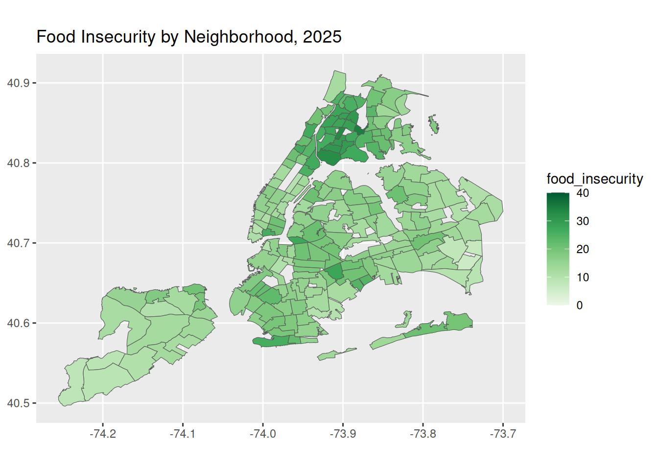
data |> filter (Year == "2024") |> ggplot() +
  geom_sf(aes(fill = food_insecurity)) +
  scale_fill_distiller(palette = "Reds", direction = 1, limits = c(0, 40), breaks = seq(0, 40, by = 10)) +
  labs(title = "Food Insecurity by Neighborhood, 2024")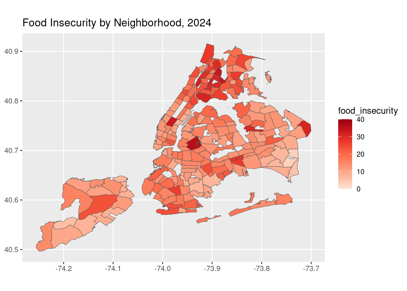
data |> filter (Year == "2023") |> ggplot() +
  geom_sf(aes(fill = food_insecurity)) +
  scale_fill_distiller(palette = "Blues", direction = 1, limits = c(0, 40), breaks = seq(0, 40, by = 10)) +
  labs(title = "Food Insecurity by Neighborhood, 2023")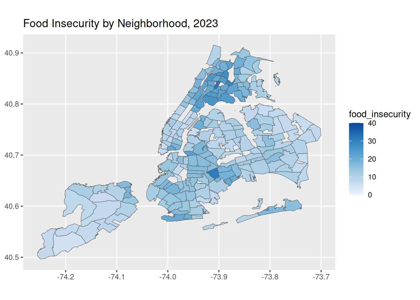
data |> ggplot(aes(x = unemployment_rate, y = food_insecurity)) + geom_point(aes(color = Year))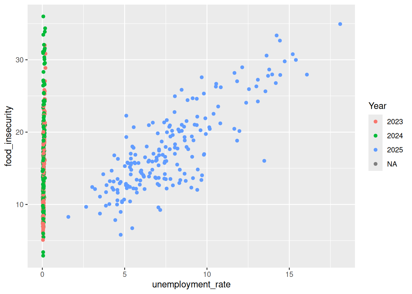
data |> filter (Year == "2024" | Year == "2023") |> ggplot(aes(x = unemployment_rate, y = food_insecurity)) + geom_point(aes(color = Year))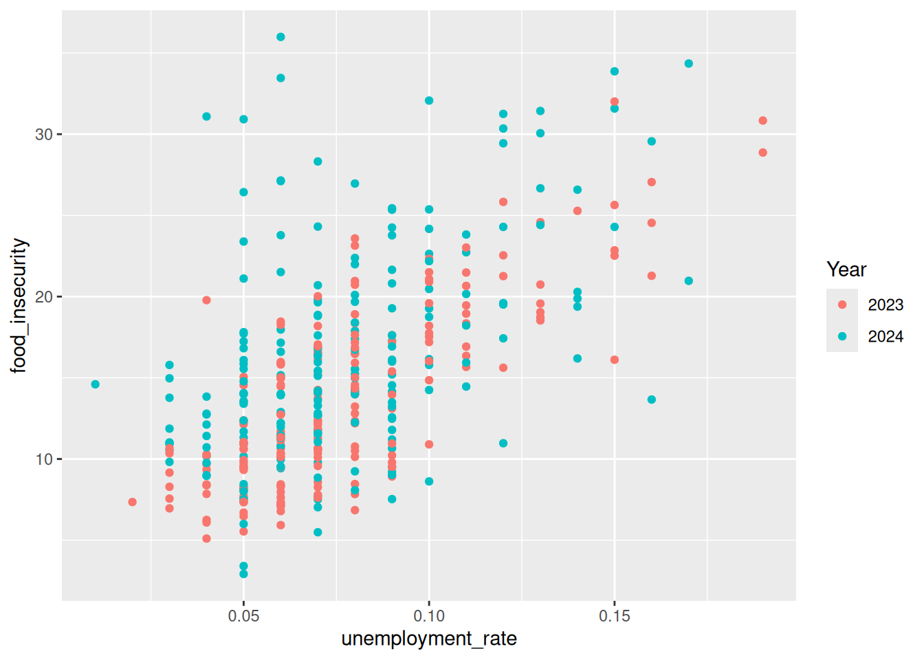
data |> filter (Year == "2025") |>
  ggplot(aes(x = unemployment_rate, y = food_insecurity)) + geom_point() + labs(title = "Food Insecurity by Neighborhood, 2025")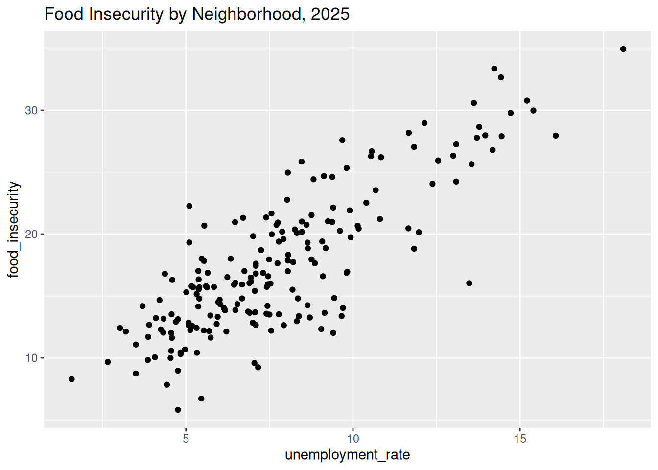
data |> filter (Year == "2025") |> group_by (BoroName) |>
  summarize (unemployment_rate_mean = mean(unemployment_rate),
             food_insecurity_mean = mean(food_insecurity)) |>
  pivot_longer(
    cols = c(unemployment_rate_mean, food_insecurity_mean),
    names_to = "indicator",
    values_to = "percentage") |>
  ggplot(aes(x = BoroName, y = percentage, fill = indicator)) +
  geom_col(position = "dodge")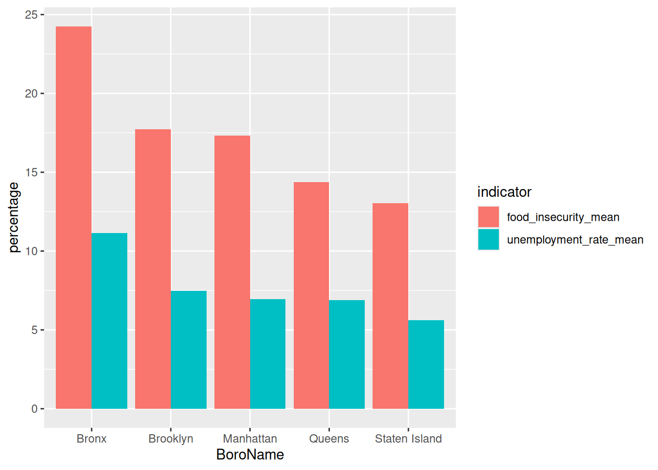
data |> filter (Year == "2025") |> group_by (BoroName) |>
  ggplot(aes(x = food_insecurity, y = reorder(BoroName, food_insecurity, median))) +
  geom_density_ridges(fill = "blue", alpha = 0.5, scale = 1) +
  ggtitle("Food Insecurity by Borough") +
  ylab("Food Insecurity Score")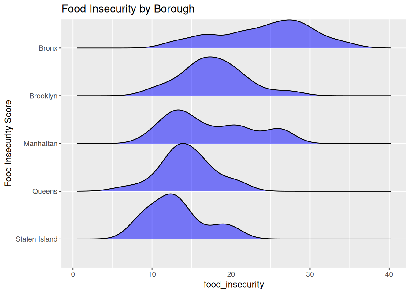
data |> filter (Year == "2025") |> group_by(BoroName) |>
  ggplot(aes(x = food_insecurity, y = reorder(BoroName, food_insecurity, median))) +
  geom_boxplot() +
  ggtitle("Food Insecurity by Borough") +
  labs(y = "Food Insecurity Score", x = "Borough")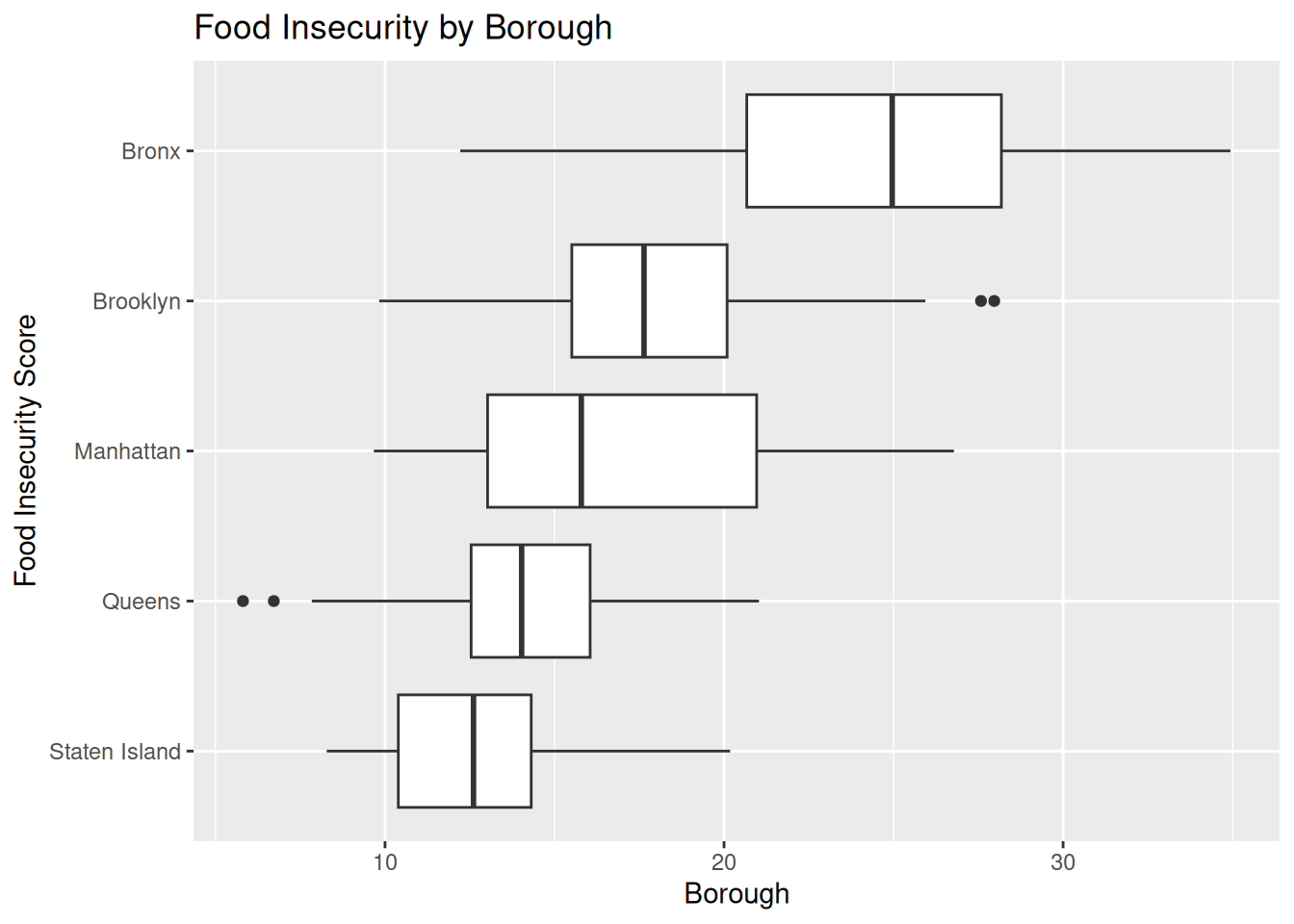
housing <- read.csv("data/Food/Housing_Database_by_2020_NTA_20260504.csv")
housing <- housing |> select(c(2:23))
data_foodhousing <- data |> left_join(housing,
    by = c("NTA2020" = "nta2020")) |> mutate(cenunits20 = parse_number(cenunits20))

data_foodhousing |> filter (Year == "2025") |> ggplot(aes(x = cenunits20, y = food_insecurity)) + geom_point()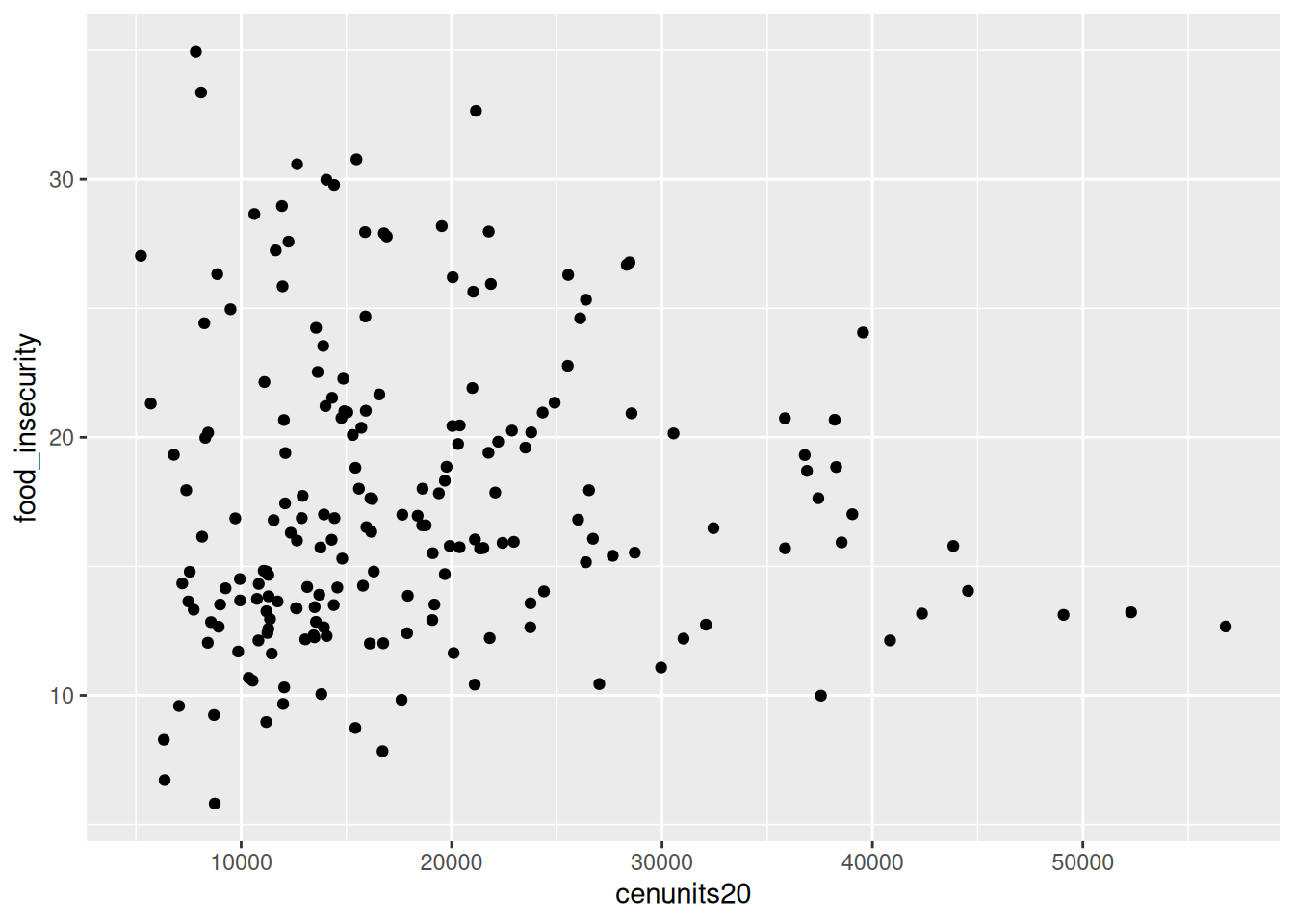
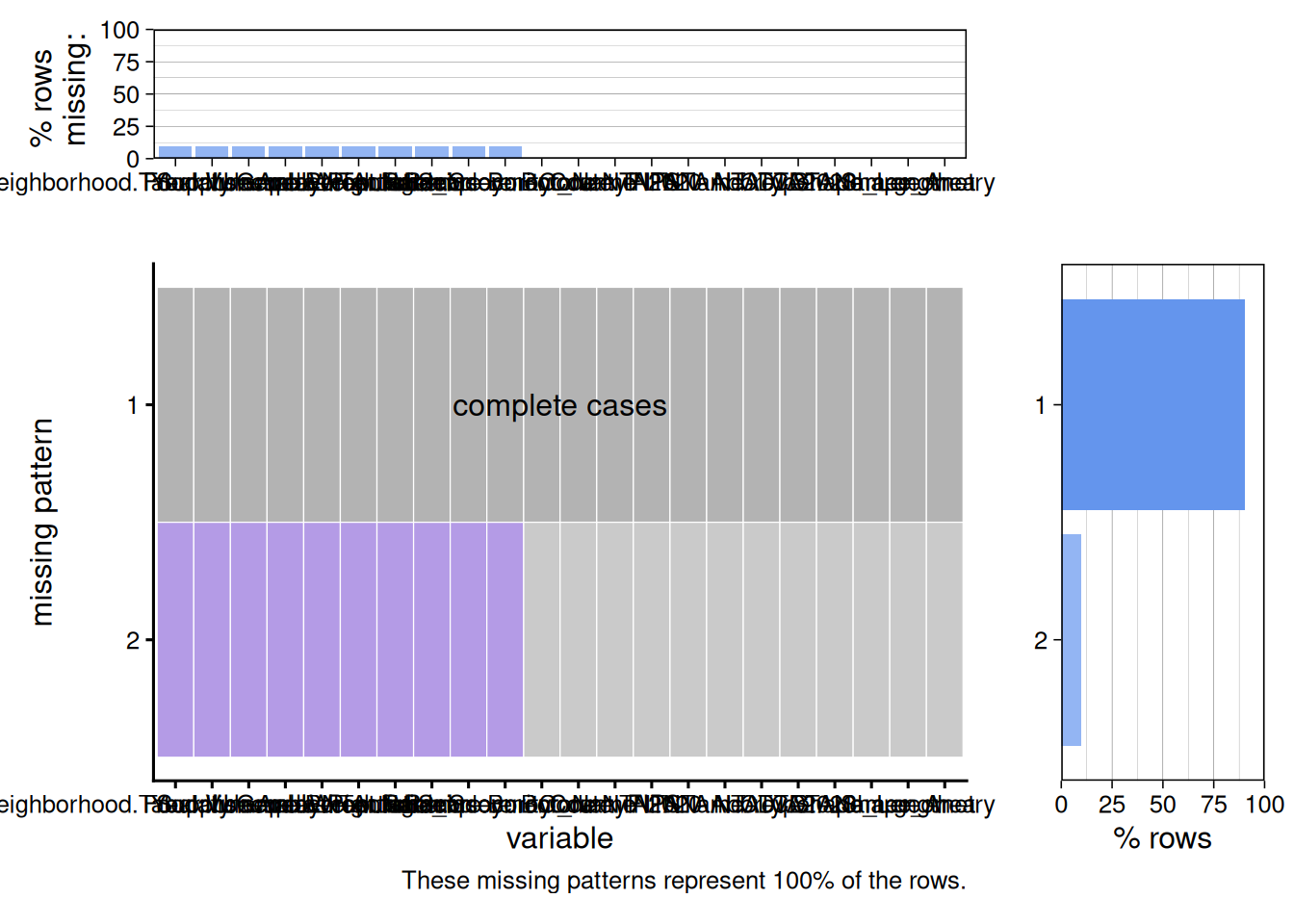
library(redav)
plot_missing(data)