8  NYC Student Feedback

Zirou Liang

8.1 Introduction

I was originally interested in a mental health-focused dataset, but found that there isn’t a large government dataset focused on residents’ psychological aspects available in NYC Open Data. However, I accessed the current dataset published by the Department of Education (DOE), which focuses on students’ feedback on their schools and includes responses indicating their satisfaction levels.

The responses are already aggregated to the school level, so instead of analyzing at an individual level, I will analyze students’ satisfaction at the school and city levels:

First, across New York City (NYC), which dimensions of school climate did students rate most and least positively? Second, do the five boroughs differ in students’ perceptions of climate, and if so, on which dimensions? Third, do the survey response rates correlate with how positively students rate their schools?

8.2 Data

library(tidyverse)

# Load the data
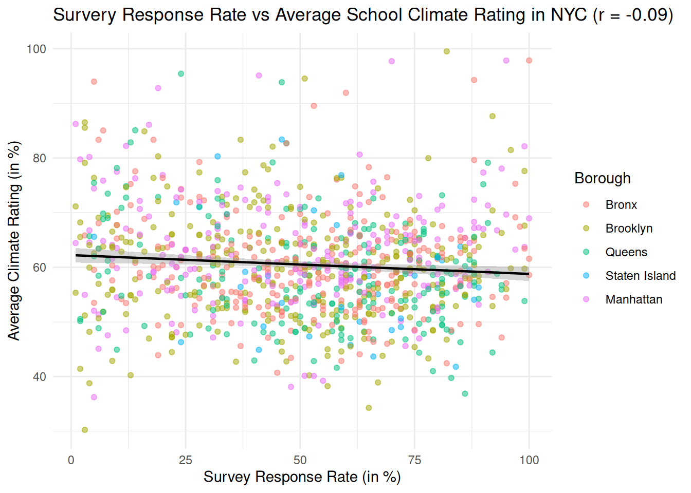
student <- read.csv("data/nyc_student_2021.csv")

# Rename the columns
names(student)[1:3] <- c("dbn", "school_name", "response_rate")

# Strip the percentage sign and convert to numeric values
percentage_col <- names(student)[3:ncol(student)]
strip_percentage <- function(col) as.numeric(str_remove(col, "%"))
student <- student |> mutate(across(all_of(percentage_col), strip_percentage))

# Parse DBN into borough
borough_lookup <- c(
  M = "Manhattan",
  X = "Bronx",
  K = "Brooklyn",
  Q = "Queens",
  R = "Staten Island"
)

student <- student |>
  mutate(borough_code = substr(dbn, 3, 3), borough = borough_lookup[borough_code]) |>
  relocate(borough_code, borough, .after = school_name)

###### Reshape question columns ######

question_col <- names(student)[6:ncol(student)]
pair_idx <- matrix(seq_along(question_col), ncol = 2, byrow = TRUE)

question_dict <- tibble(
  neg_col = question_col[pair_idx[, 1]],
  pos_col = question_col[pair_idx[, 2]],
  question_n = str_extract(neg_col, "^q\\d+"),
  question_int = as.integer(str_remove(question_n, "q"))
)

# Pair questions with their corresponding topics
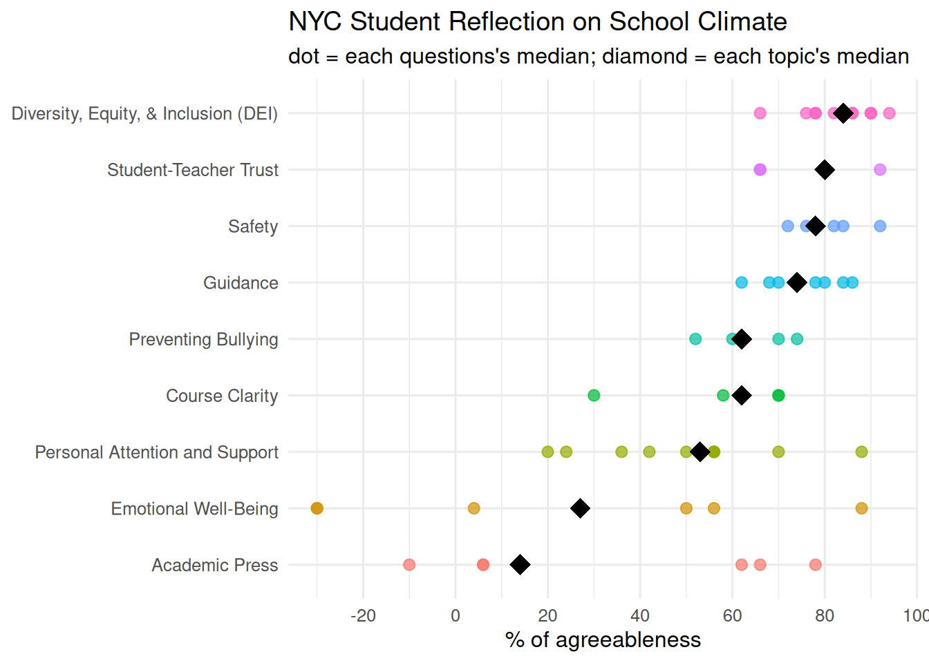
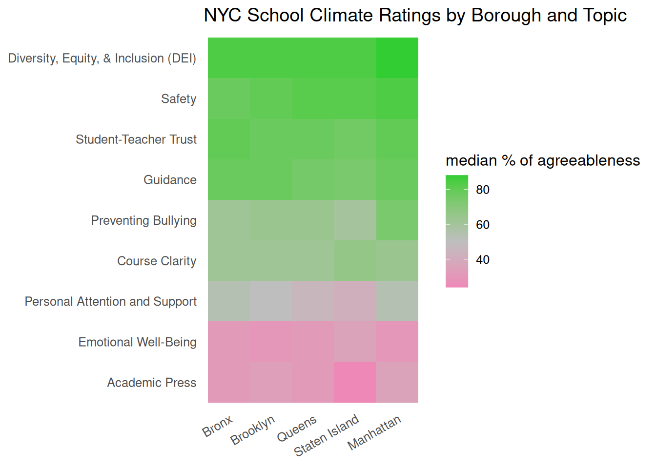
question_dict <- question_dict |> mutate(topic = case_when(
  question_int %in% c(1:10, 37) ~ "Diversity, Equity, & Inclusion (DEI)",
  question_int %in% c(11:16) ~ "Emotional Well-Being",
  question_int %in% c(17:21) ~ "Course Clarity",
  question_int %in% c(22:27, 29, 31:33) ~ "Personal Attention and Support",
  question_int %in% c(28, 39, 41:45) ~ "Academic Press",
  question_int %in% c(30, 34:36, 38) ~ "Student-Teacher Trust",
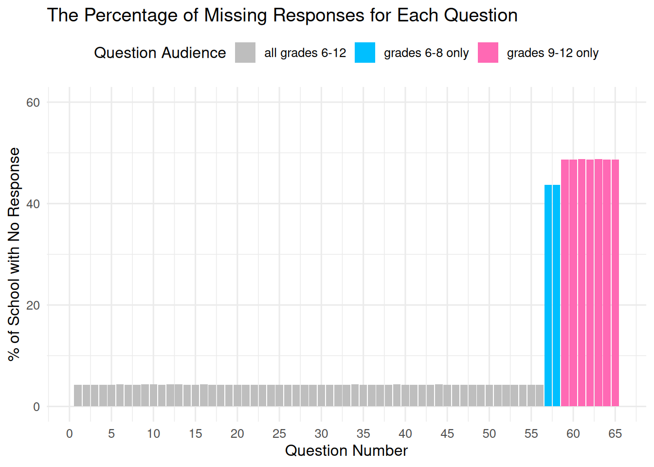
  question_int %in% c(40, 46:49, 55:56) ~ "Safety",
  question_int %in% c(50:54) ~ "Preventing Bullying",
  question_int %in% c(57:65) ~ "Guidance"
))

# Build the cleaned wide table
pos <- setNames(question_dict$pos_col, paste0(question_dict$question_n, "_pos"))
neg <- setNames(question_dict$neg_col, paste0(question_dict$question_n, "_neg"))

student_wide <- student |>
  select(dbn, school_name, borough_code, borough, response_rate, all_of(c(pos, neg)))

# Convert to long table
student_long <- student_wide |>
  pivot_longer(
    cols       = matches("^q\\d+_(pos|neg)$"),
    names_to   = c("question_n", "pole"),
    names_pattern = "(q\\d+)_(pos|neg)",
    values_to  = "percentage"
  ) |> 
  pivot_wider(names_from = pole, values_from = percentage) |>
  left_join(
    question_dict |> 
      select(question_n, question_int, topic), by = "question_n") |>
  mutate(
    net_pos = pos - neg,
    # Reverse coding so that larger values consistently indicate higher satisfaction 
    net_pos = if_else(question_int %in% c(14:16, 50:56), -net_pos, net_pos)
  )

# Select the cleaned long table
student_clean <- student_long |>
  select(school_name, borough, response_rate, question_int, topic, net_pos)

head(student_clean)

# A tibble: 6 × 6
  school_name                   borough response_rate question_int topic net_pos
  <chr>                         <chr>           <dbl>        <int> <chr>   <dbl>
1 P.S. 034 Franklin D. Rooseve… Manhat…            75            1 Dive…      26
2 P.S. 034 Franklin D. Rooseve… Manhat…            75            2 Dive…      64
3 P.S. 034 Franklin D. Rooseve… Manhat…            75            3 Dive…      80
4 P.S. 034 Franklin D. Rooseve… Manhat…            75            4 Dive…      78
5 P.S. 034 Franklin D. Rooseve… Manhat…            75            5 Dive…      80
6 P.S. 034 Franklin D. Rooseve… Manhat…            75            6 Dive…      64

8.2.1 Description

The data come from the 2021 Public Data File -Student (https://data.cityofnewyork.us/Education/2021-Public-Data-File-Student/gdx6-nrns/about_data) on NYC Open Data, published by the New York City Department of Education. The underlying survey was administered to students in grades 6-12 across NYC public schools in 2021. For privacy reasons, the published public dataset aggregates individual responses to the school level and reports, for each survey question, the percentage of respondents who selected each response category at each school. The dataset contains 1077 schools (rows) and 133 columns. The first three columns identify the school, including a District Borough Number (DBN, e.g., 01M034), the school name, and the survey response rate. The DBN encodes the school’s district (the first two characters) and borough (third character: M for Manhattan, X for Bronx, K for Brooklyn, Q for Queens, and R for Staten Island), which we will use for geographic analysis later in this chapter. The remaining 130 columns hold 65 survey questions, each split across two columns reporting the percentage of students at the “negative pole” (e.g., Strongly Disagree / Disagree) and the “positive pole” (e.g., Strongly Agree / Agree) on the response scale. The dataset is updated and published annually; I chose the 2021 dataset because it is the most recent year available on NYC Open Data.

There are two details about the question columns that are worth flagging. One is that questions q50-q56 are negative framed, asking about bullying, harassment, drug use, and gang activity, so high “positive pole” percentages on these items indicate less supportive learning environments. The other note here is that grades restrict two question blocks: q57-q58 (high school application support) are asked only of grades 6-8, and q59-q65 (college and career readiness) are asked only for grades 9-12; we will analyze the structural pattern of such missing values in the next section.

8.2.2 Missing value analysis

# Check the percentage of schools missing each question, inferred by grade-level audience

student_na <- student_clean |> mutate(grade_level = case_when(
  question_int %in% 57:58 ~ "grades 6-8 only",
  question_int %in% 59:65 ~ "grades 9-12 only",
  TRUE ~ "all grades 6-12")
  ) |>
  group_by(question_int, grade_level) |>
  summarise(percentage_na = mean(is.na(net_pos)) * 100)

ggplot(student_na, 
       aes(x = question_int, y = percentage_na, fill = grade_level)) +
  geom_col() +
  scale_x_continuous(breaks = seq(0, 65, 5)) +
  scale_y_continuous(limits = c(0, 60)) +
  scale_fill_manual(values = c(
    "all grades 6-12" = "grey",
    "grades 6-8 only" = "deepskyblue",
    "grades 9-12 only" = "hotpink"
  )) +
  labs(
    title = "The Percentage of Missing Responses for Each Question",
    x = "Question Number",
    y = "% of School with No Response",
    fill = "Question Audience"
  ) +
  theme_minimal(base_size = 12) +
  theme(legend.position = "top")

The results of missing values are unexpected: although we already knew that there would be missing responses for q57-q65 due to the grade restriction (as explained in the data description section), we found that q1-q56 have a consistent percentage of missing responses, indicating that there might be schools that didn’t submit their responses for all questions. Therefore, we will be examining schools that missed all responses in the next step:

schools_na <- student_clean |>
  group_by(school_name) |>
  filter(all(is.na(net_pos))) |>
  ungroup() |>
  distinct(school_name)

schools_na

# A tibble: 46 × 1
   school_name                                             
   <chr>                                                   
 1 Cascades High School                                    
 2 High School of Hospitality Management                   
 3 Independence High School                                
 4 Harvey Milk High School                                 
 5 High School for Law, Advocacy and Community Justice     
 6 The Lexington Academy                                   
 7 The Judith S. Kaye School                               
 8 Teachers College Community School                       
 9 Thurgood Marshall Academy for Learning and Social Change
10 P.S. X037 - Multiple Intelligence School                
# ℹ 36 more rows

As expected, we found that 46 schools failed to submit their responses. Now, let’s remove these schools from our cleaned dataset to prevent noise. Then, we will re-examine the missing value using the bar chart.

student_clean <- student_clean |>
  group_by(school_name) |>
  filter(!all(is.na(net_pos))) |>
  ungroup()

student_na <- student_clean |> mutate(grade_level = case_when(
  question_int %in% 57:58 ~ "grades 6-8 only",
  question_int %in% 59:65 ~ "grades 9-12 only",
  TRUE ~ "all grades 6-12")
  ) |>
  group_by(question_int, grade_level) |>
  summarise(percentage_na = mean(is.na(net_pos)) * 100)

ggplot(student_na, 
       aes(x = question_int, y = percentage_na, fill = grade_level)) +
  geom_col() +
  scale_x_continuous(breaks = seq(0, 65, 5)) +
  scale_y_continuous(limits = c(0, 60)) +
  scale_fill_manual(values = c(
    "all grades 6-12" = "grey",
    "grades 6-8 only" = "deepskyblue",
    "grades 9-12 only" = "hotpink"
  )) +
  labs(
    title = "The Percentage of Missing Responses for Each Question",
    x = "Question Number",
    y = "% of School with No Response",
    fill = "Question Audience"
  ) +
  theme_minimal(base_size = 12) +
  theme(legend.position = "top")

Great! Now we finally receive a cleaned dataset. There might still be a few remaining missing responses for q1-q56 that are not apparent in the bar chart, but there are too few to affect our final results, so let’s move on to analyzing our research questions.

8.3 Results

8.3.1 Question 1: across New York City (NYC), which dimensions of school climate did students rate most and least positively?

# Compute per-question and per-topic medians
questions <- student_clean |>
  group_by(topic, question_int) |>
  summarise(questions_median = median(net_pos, na.rm = TRUE))

topics <- questions |>
  group_by(topic) |>
  summarise(topics_median = median(questions_median))

# Order by topic's medians
topics <- topics |>
  mutate(topic = fct_reorder(topic, topics_median))

questions <- questions |>
  mutate(topic = factor(topic, levels = levels(topics$topic)))

# Plot the median dot plot
ggplot(questions, aes(x = questions_median, y = topic)) +
  geom_point(aes(color = topic), size = 2.5, alpha = 0.7) +
  geom_point(data = topics, aes(x = topics_median, y = topic),
             shape = 18, size = 5, color = "black") +
  scale_x_continuous(breaks = seq(-100, 100, 20)) +
  labs(
    title = "NYC Student Reflection on School Climate",
    subtitle = "dot = each questions's median; diamond = each topic's median",
    x = "% of agreeableness",
    y = NULL
  ) +
  theme_minimal(base_size = 12) +
  theme(legend.position = "none")

8.3.2 Question 2: do the five boroughs differ in students’ perceptions of climate, and if so, on which dimensions?

# Aggregate by borough and topic
borough_topic <- student_clean |>
  group_by(borough, topic) |>
  summarise(bor_top_median = median(net_pos, na.rm = TRUE))

# Order topics by their median
topics <- borough_topic |>
  group_by(topic) |>
  summarise(top_median = median(bor_top_median)) |>
  arrange(top_median) |>
  pull(topic)

# Order boroughs by their cross-topic median
boroughs <- borough_topic |>
  group_by(borough) |>
  summarise(bor_median = median(bor_top_median)) |>
  arrange(bor_median) |>
  pull(borough)

borough_topic <- borough_topic |> mutate(
  topic = factor(topic, levels = topics),
  borough = factor(borough, levels = boroughs)
)

boroughs

              X               K               Q               R               M 
        "Bronx"      "Brooklyn"        "Queens" "Staten Island"     "Manhattan" 

# Plot the heatmap
ggplot(borough_topic, 
       aes(x = borough, y = topic, fill = bor_top_median)) +
  geom_tile() +
  scale_fill_gradient2(
    low = "hotpink",
    mid = "grey",
    high = "limegreen",
    midpoint = 50,
    name = "median % of agreeableness"
  ) +
  labs(
    title = "NYC School Climate Ratings by Borough and Topic",
    x = NULL,
    y = NULL
  ) +
  theme_minimal(base_size = 12) +
  theme(
    panel.grid = element_blank(),
    axis.text.x = element_text(angle = 30, hjust = 1)
  )

8.3.3 Question 3: do the survey response rates correlate with how positively students rate their schools?

# Aggregate by school
school_avg <- student_clean |>
  group_by(school_name, borough, response_rate) |>
  summarise(pos_avg = mean(net_pos, na.rm = TRUE)) |>
  filter(!is.na(pos_avg))

# Factor in borough level (not necessary, just for better visualization)
school_avg <- school_avg |>
  mutate(borough = factor(borough, levels = boroughs))

# Compute the correlation
corr <- cor(school_avg$response_rate, school_avg$pos_avg)

# Plot the correlation graph
ggplot(school_avg, aes(x = response_rate, y = pos_avg)) +
  geom_point(aes(color = borough), alpha = 0.5, size = 1.5) +
  geom_smooth(method = "lm", color = "black", linewidth = 0.8) +
  labs(
    title = sprintf("Survery Response Rate vs Average School Climate Rating in NYC (r = %.2f)", corr),
    x = "Survey Response Rate (in %)",
    y = "Average Climate Rating (in %)",
    color = "Borough"
  ) +
  theme_minimal(base_size = 11)

8.4 Conclusion