4 NYPD Arrest Data

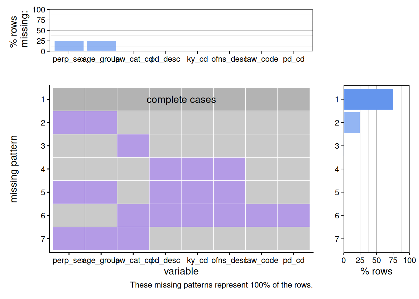
By: Jade Amaya

4.1 Introduction

I was inspired to select the NYPD Arrest (Historic) Data in lieu of other courses that discuss psychology, law, and history. I’m interested in studying the demographics of people arrested in NYC, specifically their demographics. Some questions I hope to answer are: What groups of people are being arrested the most? What are the trends of arrests? What types of crimes are people arrested for? Where are most of these arrests happening?

4.2 Data

4.2.1 Description

The data was collected by the NYPD and published by NYC’s Open Data team. The data was imported, using an API from the NYPD Arrest (Year to Date) Data set. The dataframe contains 19 columns and 1000 rows. The data is updated every year some time during mid to late April. Some limitations of this dataset is that by using an API, only 1000 rows can be imported at a time, there is no data provided that informs us whether or not these arrested people were let go, whether they were scheduled a trial, or whether some of these arrests pertain to the same individual; that some demographic information pertaining to individuals are missing; and that even though these people were arrested, cannot say for certain all actually committed the crime.

Here is a link to the dataset: link

4.2.2 Missing Value Analysis

library(redav)
df_new <- df |>
  select(starts_with(c("perp_sex", "age", "pd_d", "k", "o", "law_", "pd_c")))
colnames(df_new) <- str_remove_all(colnames(df_new), "PE")
plot_missing(df_new)

Most of the rows in the dataset contained no missing values. Above the graph shows that the second most common pattern had sex and age group missing values. The third pattern included all other columns without missing values, but the level of defense.

4.3 Results

4.3.1 Where are arrests concentrated?

#|warning: false
library(sf)
nybb <- st_read("nybb_26a/nybb.shp")

Reading layer `nybb' from data source 
  `/home/runner/work/3702project/3702project/nybb_26a/nybb.shp' 
  using driver `ESRI Shapefile'
Simple feature collection with 5 features and 4 fields
Geometry type: MULTIPOLYGON
Dimension:     XY
Bounding box:  xmin: 913175.1 ymin: 120128.4 xmax: 1067383 ymax: 272844.3
Projected CRS: NAD83 / New York Long Island (ftUS)

nybb <- nybb |>
  mutate(BoroCode = recode(BoroCode, `1` = "M", `2` = "B", `3` = "K",
                           '4' = "Q", '5' = "S")) |>
  rename(arrest_boro = BoroCode)

df <- read_csv("https://data.cityofnewyork.us/resource/uip8-fykc.csv?$limit=69000", na = c("(null)", ""))

points_sf <- df |> 
 select(longitude, latitude, arrest_boro) |> 
  na.omit() |> 
  st_as_sf(coords = c("longitude", "latitude"), crs = 4326) 
ggplot() + 
 geom_sf(data = nybb) +
  geom_sf(data = points_sf, size = .1, aes(color = arrest_boro)) +
  theme_minimal()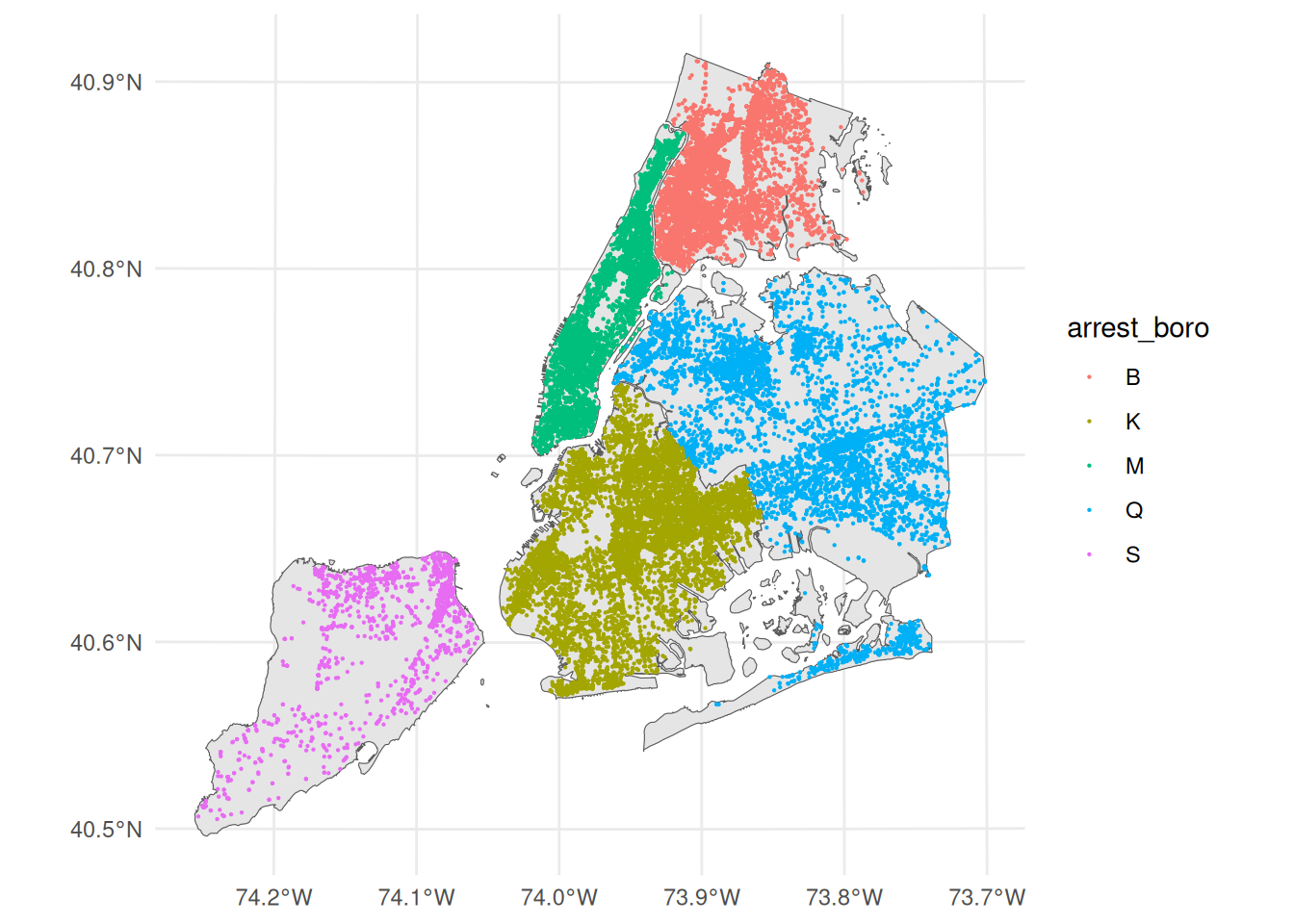

4.3.2 What are the top crimes people are allegedly arrested for?

ggplot(df, aes(y = fct_rev(fct_infreq(law_cat_cd)), fill = law_cat_cd)) + 
  geom_bar() +
 scale_fill_brewer(palette = "Set2") +
  theme_minimal() +
  labs(title = "Arrests by Crime Type",
       x = "Count",
       y = "Offense")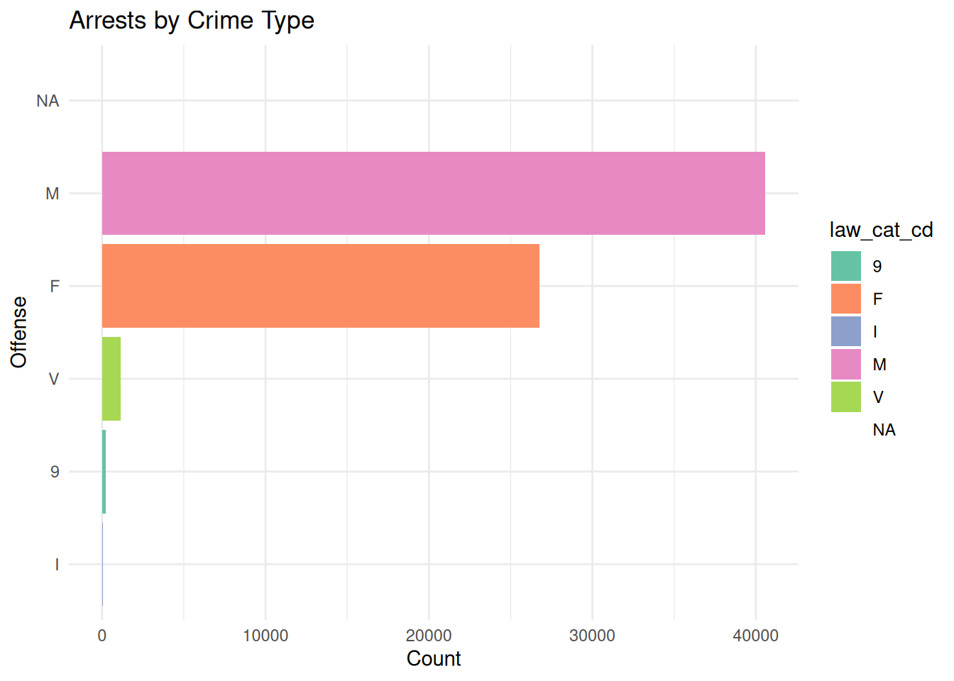

library(ggplot2)
library(forcats)

ggplot(df, aes(y = law_cat_cd)) + 
  geom_bar(aes(y = fct_rev(fct_infreq(law_cat_cd)), fill = perp_race)) +
  theme_minimal() +
 scale_fill_brewer(palette = "Set1") +
  labs(title = "Arrests in NYC by Crime", x = "count", 
       y = "Offense", fill = "Race")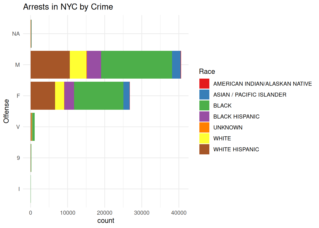

The graph represents the total counts of crime type by race, compared across gender groups, where NA was a non-specified sex. The crime codes are the following: F (felony); M (misdemeanor); V (violation); 9 (infraction).

4.3.3 Who is being disproportionately arrested?

library(ggplot2)
library(forcats)
ggplot(df, aes(y = perp_race)) + 
  geom_bar(aes(y = fct_rev(fct_infreq(perp_race)), fill = perp_sex)) +
  theme_minimal() +
  labs(title = "Arrests in NYC by Race and Gender", x = "count", y = "Race", fill = "Sex")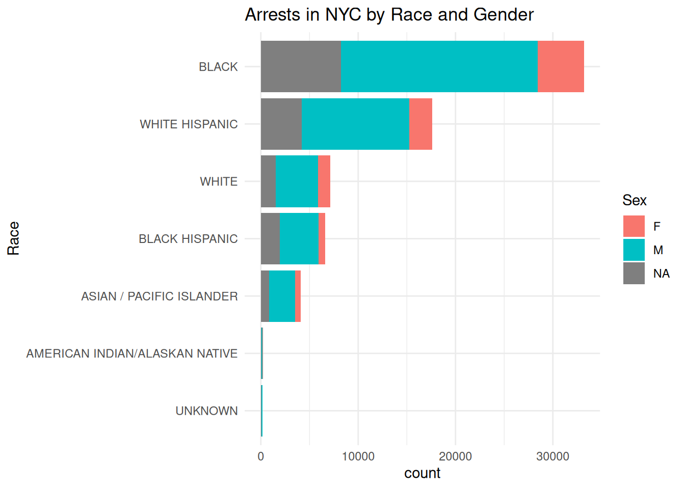

The graph above presents a bar graph of the distribution of arrests by race, each broken up by gender. People who identify as black are substantively arrested more than people who identify as another race, with white hispanics as the second highest arrested racial group. Within each racial category, people who identify as males are also arrested at substantively greater rate than people who identify as females.

library(tidyverse)
library(sf)
library(readxl)



nypp <- read_sf("nypp_25c/nypp.shp")

df <- df |>
  rename(Precinct = arrest_precinct)

newer <- left_join(nypp, df) |>
  select(c("Precinct", "perp_race", "Shape_Leng", "Shape_Area", "geometry")) |>
  group_by(perp_race, Precinct) |>
  summarise(race_count = n())

ggplot(newer) +
  geom_sf(aes(fill = perp_race)) + 
  geom_sf_text(aes(label = Precinct), size = 2, color = "white")  +
  theme_void() +
  facet_wrap(vars(perp_race))

newdata <- left_join(nypp, df) |>
  select(c("Precinct", "perp_sex", "Shape_Leng", "Shape_Area", "geometry")) |>
  filter(perp_sex == "M") |>
  group_by(Precinct) |>
  summarise(Male = n())

male <- ggplot(newdata) +
  geom_sf(aes(fill = Male)) + 
  geom_sf_text(aes(label = Precinct), size = 2,
               color = "white") +
   scale_fill_gradient(low = "darkblue", high = "lightblue",
                     na.value = "grey70") +
  theme_void()

library(patchwork)

women <- left_join(nypp, df) |>
  select(c("Precinct", "perp_sex", "Shape_Leng", "Shape_Area", "geometry")) |>
  filter(perp_sex == "F") |>
  group_by(Precinct) |>
  summarise(Female = n())

female <- ggplot(women) +
  geom_sf(aes(fill = Female)) + 
  geom_sf_text(aes(label = Precinct), size = 2,
               color = "white") +
   scale_fill_gradient(low = "darkblue", high = "lightblue",
                     na.value = "grey70") +
  theme_void()

female | male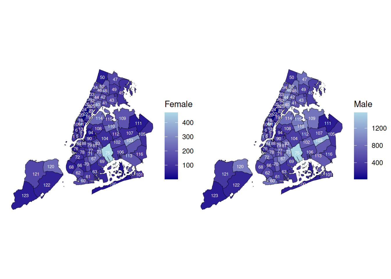

At a glance, the maps look similar when comparing male and female arrestees across precincts. However, we already established that males arrests were substantively larger than the amount of female arrests. However, if you look at the colors, you can see they are similar in color, which may suggest there is some sort of underlying pattern beyond gender. In other words, there is not a strong association between gender and location, because it looks like both male and females are arrested at higher rates in certain precincts. Maybe there is some other variable that can explain why within the precincts that are lighter result in higher arrest counts of each gender.

white <- left_join(nypp, df) |>
  select(c("Precinct", "perp_race", "Shape_Leng", "Shape_Area", "geometry")) |>
  filter(perp_race == "WHITE") |>
  group_by(Precinct) |>
  summarise(
    white_count = n())

black <- left_join(nypp, df) |>
  select(c("Precinct", "perp_race", "Shape_Leng", "Shape_Area", "geometry")) |>
  filter(perp_race == "BLACK") |>
  group_by(Precinct) |>
  summarise(
    black_count = n())

g1 <- ggplot(white) +
  geom_sf(aes(fill = white_count)) + 
  geom_sf_text(aes(label = Precinct), size = 2,
               color = "white")  +
  labs(fill = "White Arrestees") +
  theme_void()

g2 <- ggplot(black) +
  geom_sf(aes(fill = black_count)) + 
  geom_sf_text(aes(label = Precinct), size = 2,
               color = "white")  +
  labs(fill = "Black Arrestees") +
  theme_void()

library(patchwork)
g1 + g2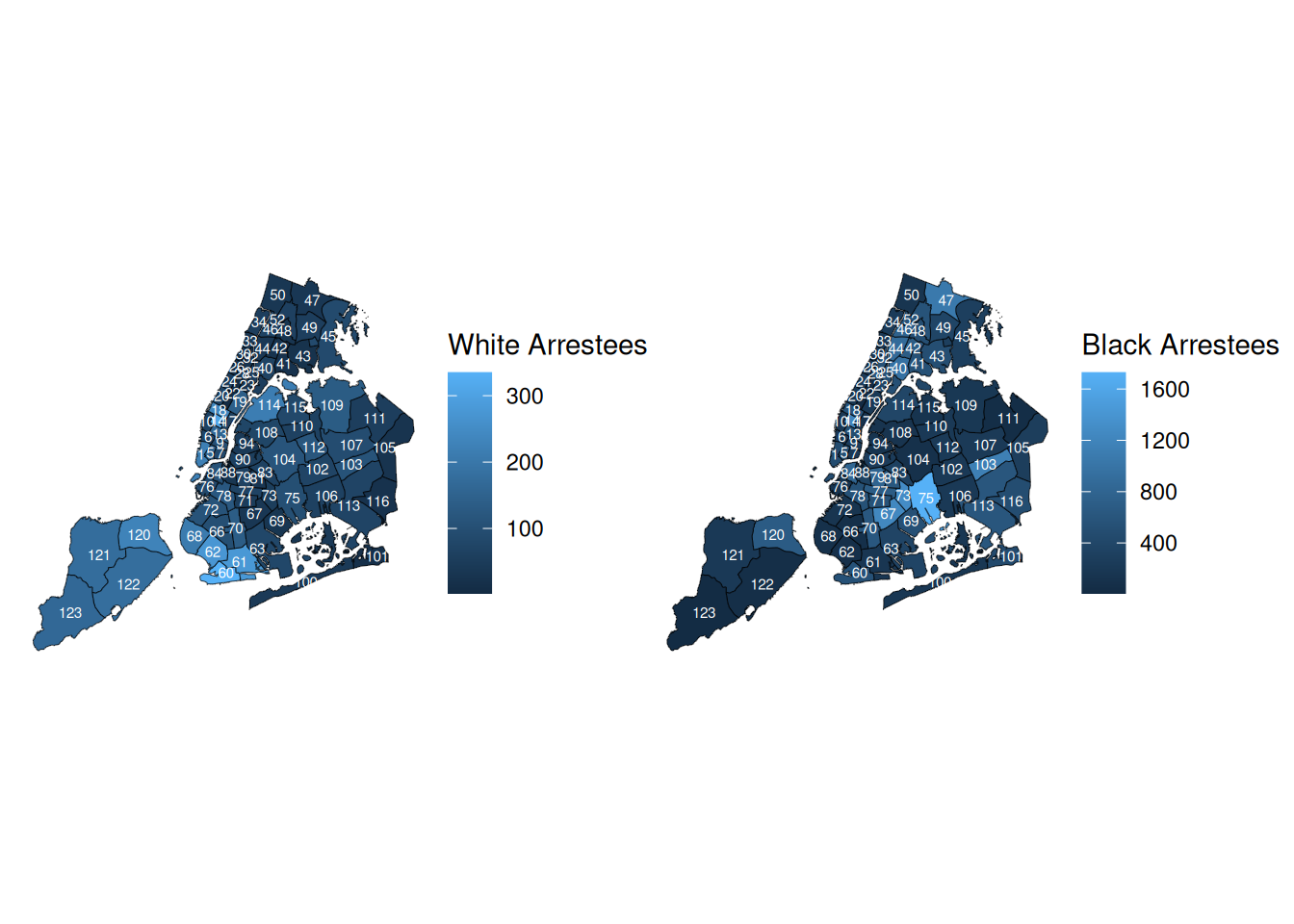

race_counts <- newer |>
  group_by(Precinct, perp_race) |>
  mutate(count = n()) |>
  ungroup()

prop_data <- race_counts |>
  group_by(Precinct) |>
  mutate(prop = count / sum(count))

ggplot(prop_data) +
  geom_sf(aes(fill = prop)) +
  geom_sf_text(aes(label = Precinct), size = 2, color = "white") +
  facet_wrap(~perp_race) +
  theme_minimal()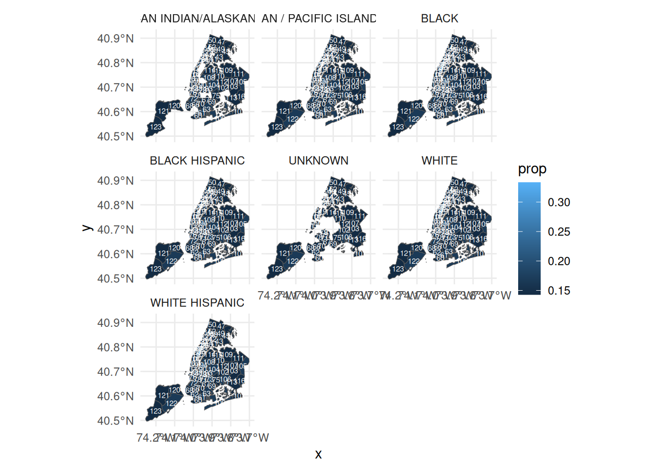

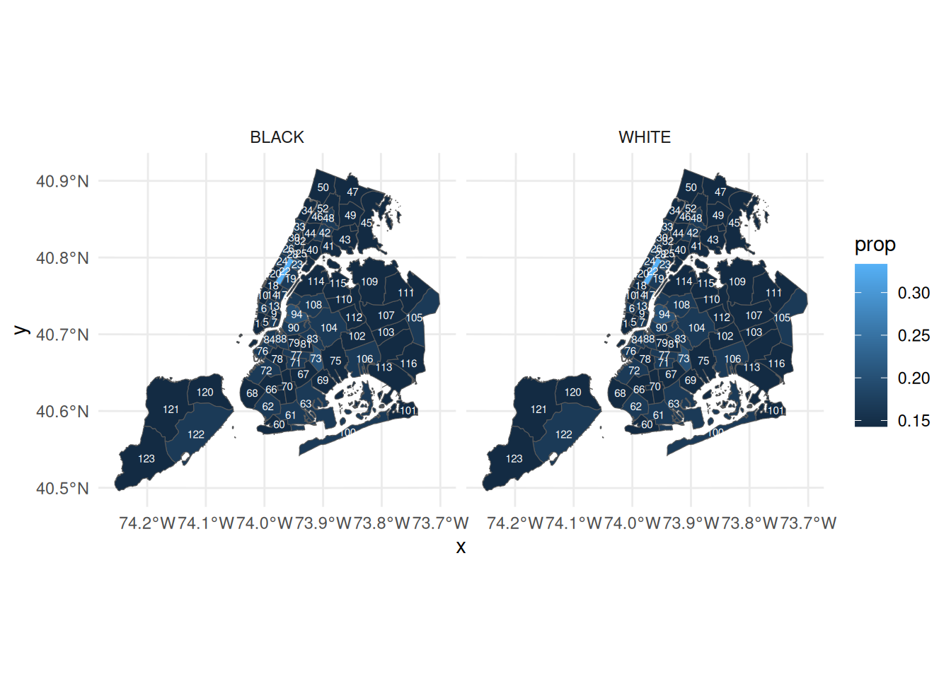
filtered_data <- prop_data |> 
  filter(perp_race %in% c("WHITE", "BLACK"))

ggplot(filtered_data) +
  geom_sf(aes(fill = prop)) +
  geom_sf_text(aes(label = Precinct), size = 2, color = "white") +
  facet_wrap(~perp_race) +
  theme_minimal()