17 Time Series with Missing Data
 This chapter originated as a community contribution created by sdt2134
This page is a work in progress. We appreciate any input you may have. If you would like to help improve this page, consider contributing to our repo.
17.1 Overview
For data scientists, data preparation could easily be the second most frustrating task, right after explaining their models to other departments. Missing value treatment is a key part of data preparation and knowing how to handle it well can reduce the excruciating pain one feels after seeing a poor RMSE. The chapter on missing data talks about some of the ways you could handle missing data in your dataset; this walkthrough takes it further focusing specifically on timeseries data.
17.2 Motivation
Why should you care when you have mean, median & mode?
You should care because time series problems are not that straight-forward. Most often time series are accompanied by forecasting tasks and most algorithms won’t allow missing data. Imputation using mean, median & mode might hide trends or seasonal patterns whereas removing missing data points altogether might reduce information contained in other features for those cases. ImputeTS in R provides a bunch of functions to visualize and approximate missing values with high precision.
But first you must ask yourself two questions:
- Is there any identifiable reason for it?
- Are they missing at random?
Is there any identifiable reason for it? Let’s take the example of a bakery. You are forecasting daily cake sales and find missing data is linked to holidays. How to impute? One way could be to fill with zeroes and create a flag that could help your forecasting algorithm understand this pattern.
If sales are missing if your cakes were out of stock or the baker was on leave such flags won’t work as you cannot predict these events in the future. Imputation is ideal for treating such cases.
What if they are missing at random? You have only one option - imputation.
Let’s go through a time series exercise where we have to decompose it when missing values are present.
Dataset : a10 “Monthly anti-diabetic drug sales in Australia from 1992 to 2008” For this walkthrough we will use two copies of the a10 dataset.
Here’s the original dataset from the fpp package
complete_a10 <- fpp::a10Let’s create missing values and check the performance of various imputation functions on hidden values.
set.seed(134)
missatrand_a10 <- complete_a10
missatrand_a10[sample(length(complete_a10),0.2*length(complete_a10))] <- NA
17.2.0.1 Let’s analyse this timeseries graphically
plot(missatrand_a10)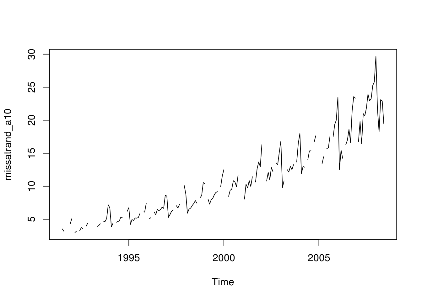
Looks like the series has multiplicative seasonality. Let’s transform it into additive to see if seasonality appears more clearly.
plot(log(missatrand_a10))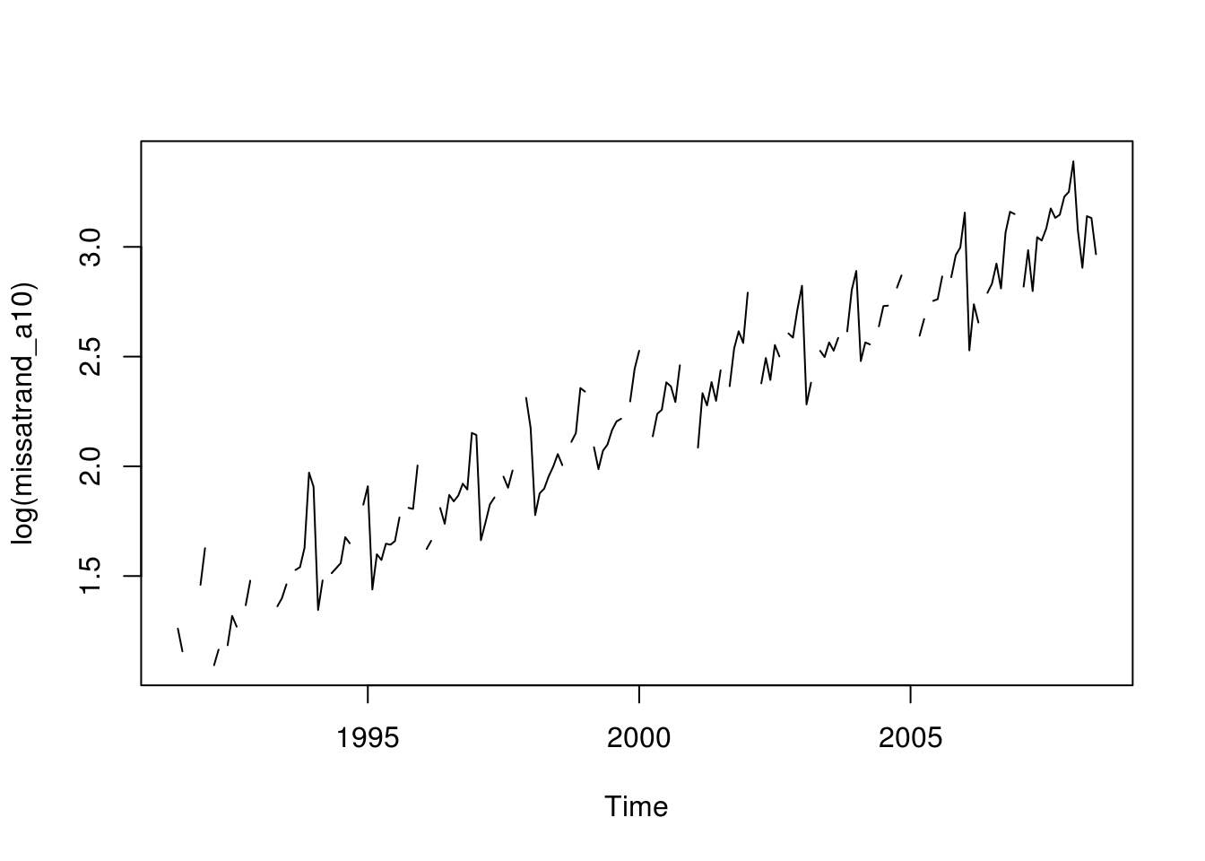
Wow, it shows a clear seasonal pattern with an increasing trend.
17.2.0.2 What if we decompose it into into its components
plot(decompose(missatrand_a10, type = "multiplicative"))## Error in na.omit.ts(x): time series contains internal NAsNot so fast. As mentioned above, we must treat the missing values before we do this. Enough said let’s impute this missing piece into our toolkit!
17.3 Visualizing missing values
library(imputeTS)

plotNA.distribution(missatrand_a10)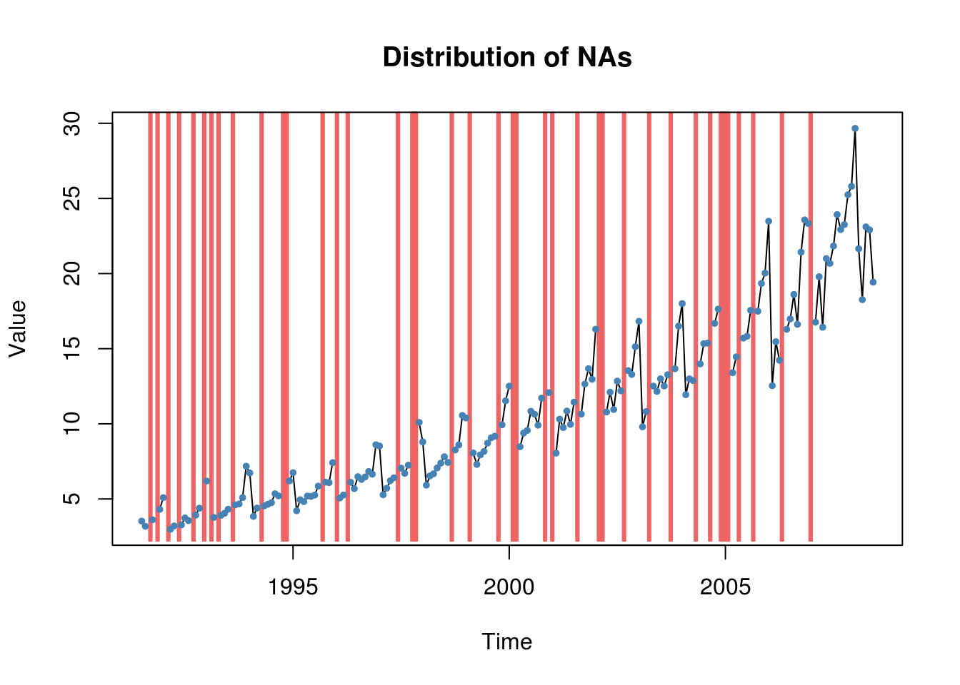
Let’s get a summary of the missing values.
statsNA(missatrand_a10)## [1] "Length of time series:"
## [1] 204
## [1] "-------------------------"
## [1] "Number of Missing Values:"
## [1] 40
## [1] "-------------------------"
## [1] "Percentage of Missing Values:"
## [1] "19.6%"
## [1] "-------------------------"
## [1] "Stats for Bins"
## [1] " Bin 1 (51 values from 1 to 51) : 13 NAs (25.5%)"
## [1] " Bin 2 (51 values from 52 to 102) : 8 NAs (15.7%)"
## [1] " Bin 3 (51 values from 103 to 153) : 10 NAs (19.6%)"
## [1] " Bin 4 (51 values from 154 to 204) : 9 NAs (17.6%)"
## [1] "-------------------------"
## [1] "Longest NA gap (series of consecutive NAs)"
## [1] "3 in a row"
## [1] "-------------------------"
## [1] "Most frequent gap size (series of consecutive NA series)"
## [1] "1 NA in a row (occuring 29 times)"
## [1] "-------------------------"
## [1] "Gap size accounting for most NAs"
## [1] "1 NA in a row (occuring 29 times, making up for overall 29 NAs)"
## [1] "-------------------------"
## [1] "Overview NA series"
## [1] " 1 NA in a row: 29 times"
## [1] " 2 NA in a row: 4 times"
## [1] " 3 NA in a row: 1 times"Are there any patterns in missingness, how many consecutive NA’s are there (gapsize), and how many missing values are accounted by a specific gapsize?
plotNA.gapsize(missatrand_a10)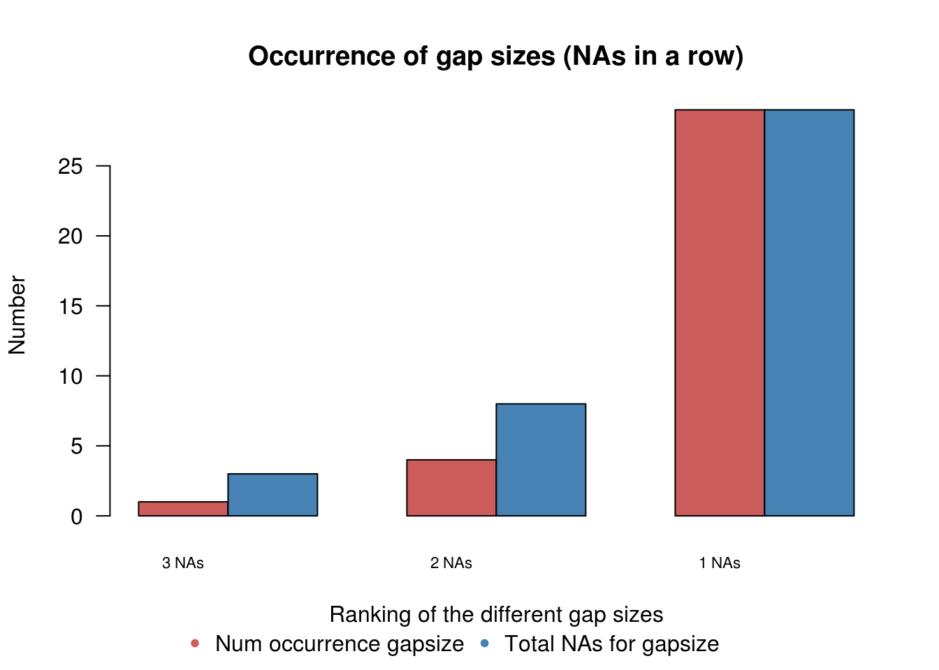
17.4 Imputing missing values
17.4.1 Generic methods : independent of time series’ temporal properties
17.4.1.1 Mean, median and mode
This is a straight forward and simple method for interpolation. But given we are imputing the missing value by calculating the mean, we end up losing information around the trend and seasonality, leading to huge errors in imputation. Because of this reason, this method is best suited for data that is stationary. This function also allows us to use other measures like median and mode.
17.4.1.1.0.1 Method 1
imp <- na.mean(missatrand_a10)
p1<-as.tibble(cbind(Date = as.yearmon(time(missatrand_a10)),
                missatrand = missatrand_a10,complete_a10 = complete_a10,imputed_val = imp))%>%
                mutate(imputed_val = ifelse(is.na(missatrand),imputed_val,NA),
                       complete_a10 = ifelse(is.na(missatrand),complete_a10,NA)
                       )%>%
  ggplot(aes(x=Date)) +
    #geom_line(aes(y=missatrand),color="red")+
    geom_line(aes(y=missatrand),color = "black")+
    geom_point(aes(y=imputed_val),color = "blue")+
    geom_point(aes(y=complete_a10),color = "red")+
    ylab("Anti-diabetic drug sales")+
    ggtitle("Imputed values (Blue); Real values (Red) ")+
    theme(plot.title = element_text(size = 10))

p2 <- ggplot() +
  geom_line(aes(y = complete_a10-imp, x = as.yearmon(time(missatrand_a10)) )) +
  ylim(-10,10) +
  ylab("Errors")+
  xlab("Date")+
  ggtitle(paste("Errors in imputation"))+
  theme(plot.title = element_text(size = 10))

grid.arrange(p1, p2, ncol=2,top="Interpolation using mean")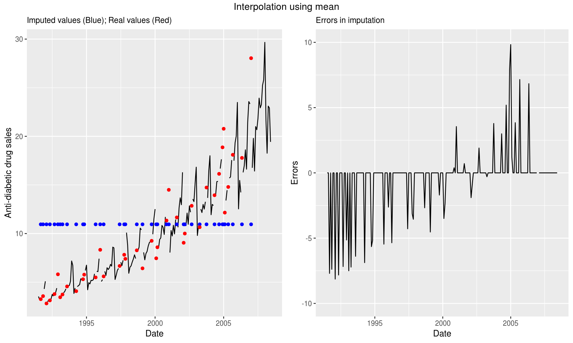
17.4.1.2 Moving Averages
As this function calculates moving averages based on the last n observations, it will generally be performing better than the last method. Moving averages work well when data has a linear trend. This function also allows us to use linear-weighted and exponentially-weighted moving averages.
17.4.1.2.0.1 Method 2
imp <- na.ma(missatrand_a10)
p1<-as.tibble(cbind(Date = as.yearmon(time(missatrand_a10)),
                missatrand = missatrand_a10,complete_a10 = complete_a10,imputed_val = imp))%>%
                mutate(imputed_val = ifelse(is.na(missatrand),imputed_val,NA),
                       complete_a10 = ifelse(is.na(missatrand),complete_a10,NA)
                       )%>%
  ggplot(aes(x=Date)) +
    #geom_line(aes(y=missatrand),color="red")+
    geom_line(aes(y=missatrand),color = "black")+
    geom_point(aes(y=imputed_val),color = "blue")+
    geom_point(aes(y=complete_a10),color = "red")+
    ylab("Anti-diabetic drug sales")+
    ggtitle("Imputed values (Blue); Real values (Red) ")+
    theme(plot.title = element_text(size = 10))

p2 <- ggplot() +
  geom_line(aes(y = complete_a10-imp, x = as.yearmon(time(missatrand_a10)) )) +
  ylim(-10,10) +
  ylab("Errors")+
  xlab("Date")+
  ggtitle(paste("Errors in imputation"))+
  theme(plot.title = element_text(size = 10))

grid.arrange(p1, p2, ncol=2,top="Interpolation using n-Moving Averages")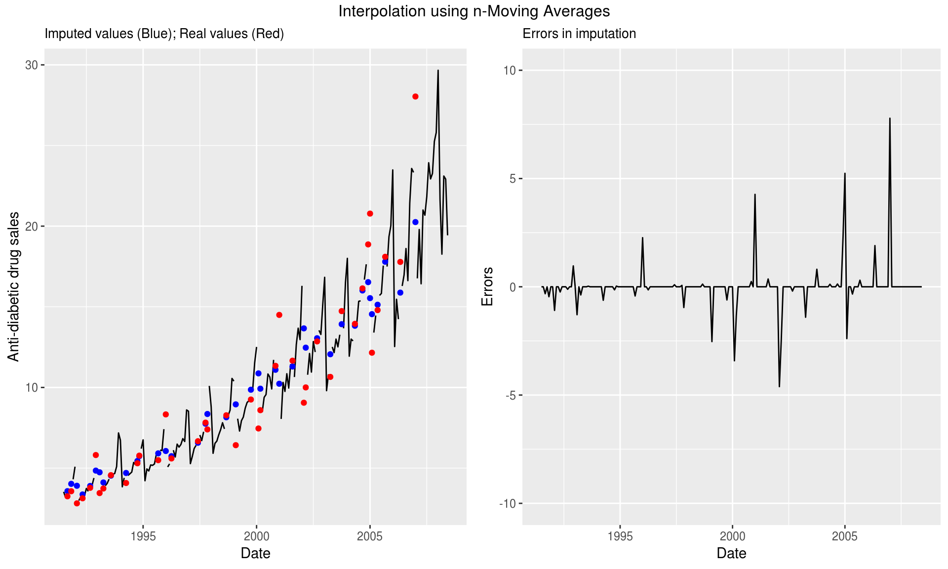
17.4.2 Time series specific methods
17.4.2.1 Kalman smoothing with auto.arima
This is a more advanced function for interpolation and requires higher computation time. It uses Kalman Smoothing on ARIMA model to impute the missing values. Structural time series models are another type of model that can be used to impute missing values using this function .
17.4.2.1.0.1 Method 3
imp <- na.kalman(missatrand_a10,model = "auto.arima")
p1<-as.tibble(cbind(Date = as.yearmon(time(missatrand_a10)),
                missatrand = missatrand_a10,complete_a10 = complete_a10,imputed_val = imp))%>%
                mutate(imputed_val = ifelse(is.na(missatrand),imputed_val,NA),
                       complete_a10 = ifelse(is.na(missatrand),complete_a10,NA)
                       )%>%
  ggplot(aes(x=Date)) +
    #geom_line(aes(y=missatrand),color="red")+
    geom_line(aes(y=missatrand),color = "black")+
    geom_point(aes(y=imputed_val),color = "blue")+
    geom_point(aes(y=complete_a10),color = "red")+
    ylab("Anti-diabetic drug sales")+
    ggtitle("Imputed values (Blue); Real values (Red) ")+
    theme(plot.title = element_text(size = 10))

p2 <- ggplot() +
  geom_line(aes(y = complete_a10-imp, x = as.yearmon(time(missatrand_a10)) )) +
  ylim(-10,10) +
  ylab("Errors")+
  xlab("Date")+
  ggtitle(paste("Errors in imputation"))+
  theme(plot.title = element_text(size = 10))

grid.arrange(p1, p2, ncol=2,top="Interpolation using Auto.arima")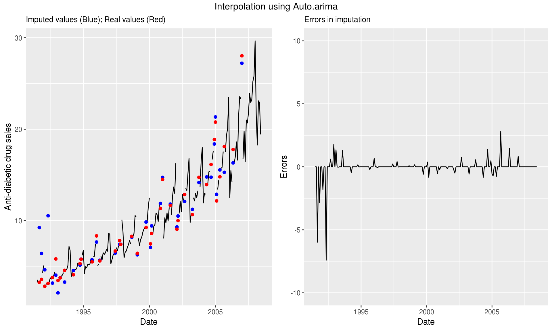
17.4.2.2 Seasonal splitting
This function interpolates missing values by splitting the data by seasons and performing imputation on the resulting datasets. Another similar function that works based on the seasonality component in this package is na.seadec() which deseasonalizes the data, performs imputation, and adds the seasonal component back again.
17.4.2.2.0.1 Method 4
imp <- na.seasplit(missatrand_a10)
p1<-as.tibble(cbind(Date = as.yearmon(time(missatrand_a10)),
                missatrand = missatrand_a10,complete_a10 = complete_a10,imputed_val = imp))%>%
                mutate(imputed_val = ifelse(is.na(missatrand),imputed_val,NA),
                       complete_a10 = ifelse(is.na(missatrand),complete_a10,NA)
                       )%>%
  ggplot(aes(x=Date)) +
    #geom_line(aes(y=missatrand),color="red")+
    geom_line(aes(y=missatrand),color = "black")+
    geom_point(aes(y=imputed_val),color = "blue")+
    geom_point(aes(y=complete_a10),color = "red")+
    ylab("Anti-diabetic drug sales")+
    ggtitle("Imputed values (Blue); Real values (Red) ")+
    theme(plot.title = element_text(size = 10))

p2 <- ggplot() +
  geom_line(aes(y = complete_a10-imp, x = as.yearmon(time(missatrand_a10)) )) +
  ylim(-10,10) +
  ylab("Errors")+
  xlab("Date")+
  ggtitle(paste("Errors in imputation"))+
  theme(plot.title = element_text(size = 10))

grid.arrange(p1, p2, ncol=2,top="Seasonally splitted interpolation")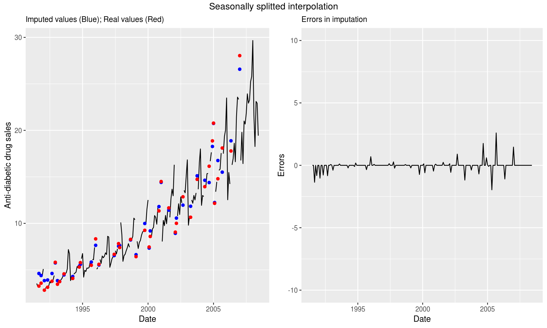
with