43 Section 3.Time series visualization with ggplot and ggplot2

The first method to visualize stock price is to use line graphs in ggplot. The function geom_line creates lines connecting observations ordered by x value. We create visualization for both raw data and log_transfomred data for GOOG stock price.

Practical Example:
Use ggplot2 to create visualization for both raw data and log_transfomred data for GOOG stock price with the line graph.
Coding Time:

#line plot for stock price raw data
ggplot(s_price, aes(x = index(s_price), y = s_price)) +
    geom_line(color = '#4E84C4', size=0.2) + 
    ggtitle('GOOG stock price, 2021-2022') + xlab('Date') + ylab('Price') + 
    theme(plot.title = element_text(hjust = 0.5)) + 
    scale_x_date(date_labels = '%y-%m', date_breaks = '3 months')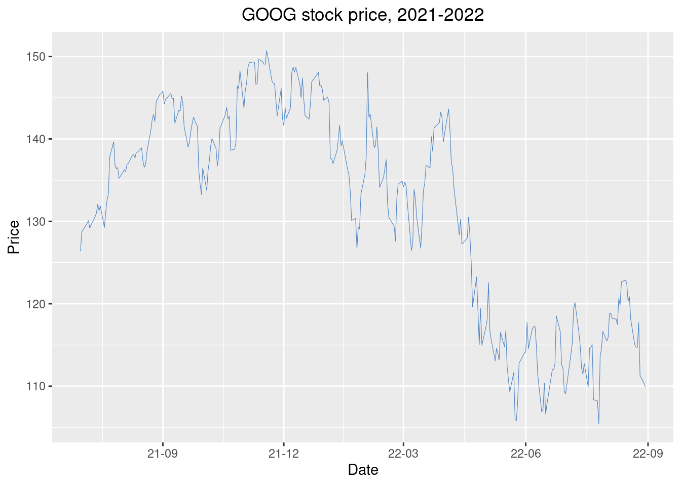

#line plot for log Transformed GOOGstock price 
ggplot(ts_goog, aes(x = index(ts_goog), y = ts_goog)) +
    geom_line(color = '#4E84C4', size=0.2) + 
    ggtitle('Log_transformed GOOG stock price, 2021-2022') + xlab('Date') + ylab('Price') + 
    theme(plot.title = element_text(hjust = 0.5)) + 
    scale_x_date(date_labels = '%y-%m', date_breaks = '3 months')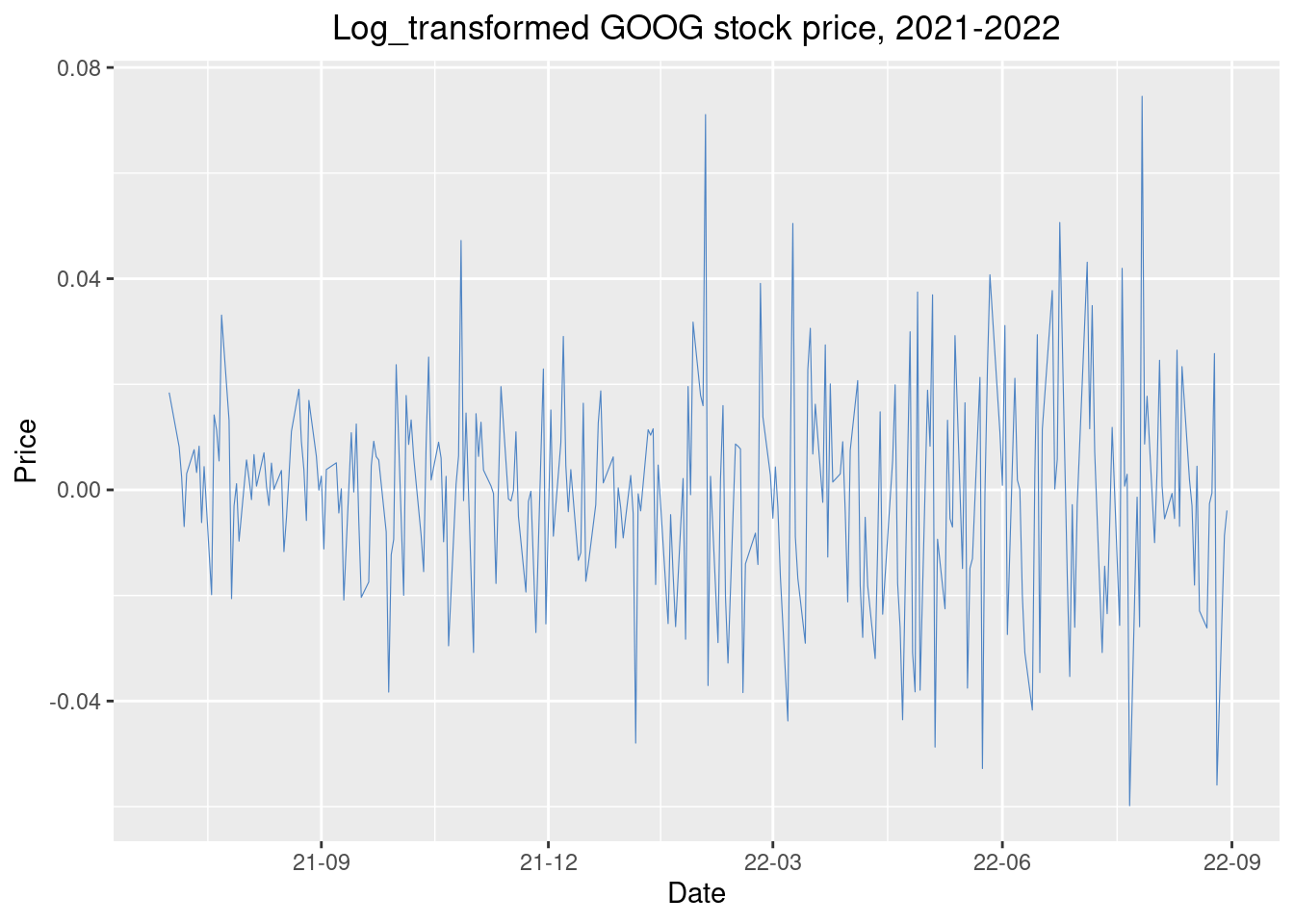

From two plots, we observe that the log_transformed stock price better represents the change in perentage for stock prices. We will use the log_transformed stock data in further visualizations.

Practical Example:
Why don’t we visualized the Google stock price and Amazon stock price on the same graph for comparison? Code below create line plots for GOOG and AMZN log_transformed stock prices at same plot by adding two geom_line.

Coding Time:

ts_bind <- cbind(ts_goog, ts_amzn)
ggplot(ts_bind, aes(x = index(ts_bind))) +
    geom_line(aes(y = GOOG.Adjusted), color = '#4E84C4', size=0.2) + 
    geom_line(aes(y = AMZN.Adjusted), color = 'red', size=0.2) + 
    ggtitle('GOOG and AMZN log_transformed stock price, 2021-2022') + xlab('Date') + ylab('Price') + 
    theme(plot.title = element_text(hjust = 0.5)) + 
    scale_x_date(date_labels = '%y-%m', date_breaks = '3 months')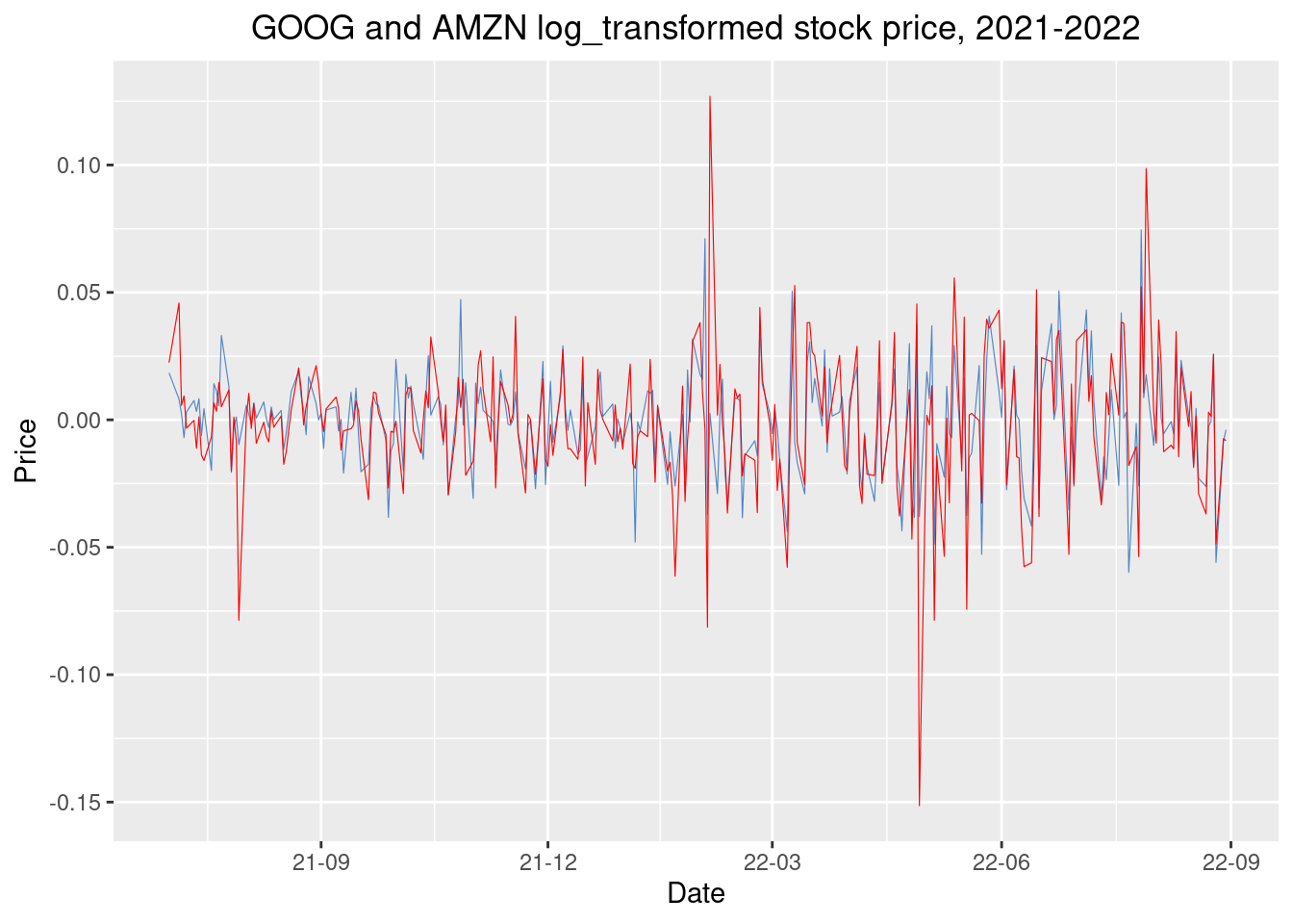

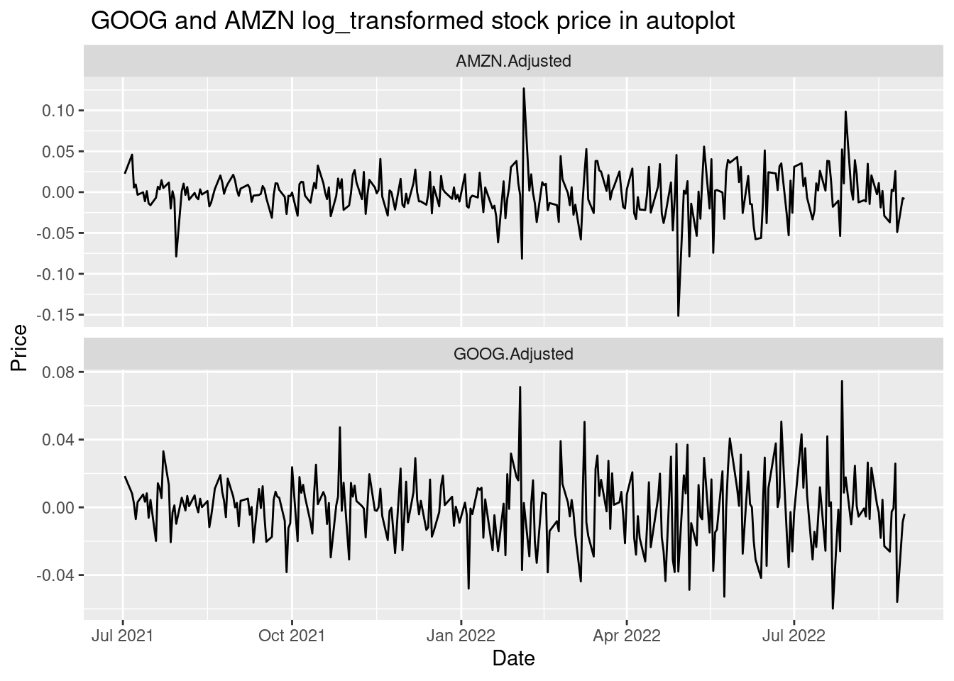
Another way to create ts visualization is to use autoplot function in ggplot2. The function autoplot() in ggplot2 provides a simple and direct plot for a particular object.

Practical Example:
Use function autoplot() to visualized the Google and Amazon log_transformed stock price.
Coding Time:

autoplot(ts_bind)  + 
    ggtitle(' GOOG and AMZN log_transformed stock price in autoplot') + xlab('Date') + ylab('Price')