Chapter 52 A basic Introduction to Markov Chain Monte Carlo Method in R
Qiran Li
52.1 1. Introduction
It is often not possible to understand (or learn) complicated probability distribution by theoretical analysis. In that scenario, one convenient way to learn about the probability distribution is to simulate from that particular distribution. Markov Chain Monte Carlo (MCMC) is probably the most popular way for the simulation purpose. It has wide application in statistics, data science, and machine learning. In this tutorial, I would first explain the theory of MCMC, and then provide my own implementation of this method in R as well as useful graphs for explanation. The purpose of this community contribution tutorial is to help people understand this tough but useful method.
As we can see from the name of MCMC method, it contains two parts. One is related to Monte Carlo Simulation (MC) Method; the other is associated with Markov chain. Therefore, It would be nature to discuss MCMC by first introducing these two related methods.
52.2 2. Markov Chain Simulation Method
The name of Monte Carlo was derived from a casino. The earliest applications of Monte Carlo Method were designed to solve some complex summation or integration problems. Suppose we want to solve the integration problem: \(\int_{a}^{b} f(x) dx\), but it’s hard to find the explicit form of \(f(x)\). One easy way of solving this problem is: find a \(x_0\) between a and b and use \(f(x_0)\) to represent all the values of \(f(x)\) inside a and b. Then the answer would be \((b - a)f(x_0)\). However, using one value to represent all the values between a and b is a broad assumption. We could also use n values \((x_0,x_1,x_2,x_3,...,x_{n-1})\) between a and b instead, thus the solution would be \(\frac{b-a}{n} \sum_{i=0}^{n - 1} f(x_i)\). Here we also made an assumption that x is uniformly distributed on [a,b]. If we know \(x\)’s distribution \(p(x)\) on [a,b], the answer would become \(\frac{1}{n} \sum_{i=0}^{n - 1} \frac {f(x_i)}{p(x_i)}\). Therefore, as long as we know the distribution of x on the interval, we could get an accurate estimate of the integral.
52.3 3. Acceptance-Rejection Sampling
If the probability distribution of {x} is found, we need to get n samples based on this probability distribution and bring them into the Monte Carlo Simulation Method formula to solve it. How do we get the n samples based on the probability distribution? For common distributions like Uniform, F, Beta, Gamma distributions, we could use random number generator to get samples. However, for complicated distribution \(p(x)\) that we could not directly sample, we need to use Acceptance-Rejection Sampling method. The process contains:
Set a common probability distribution function \(q(x)\) that is convenient for sampling, set a constant \(k\) so that \(p(x)\) is always below \(kq(x).\)
Get a sample \(z_0\) of \(q(x)\).
Sample a value u from a uniform distribution \((0, kq(z_0))\). If u falls below \(kq(z)\) and above \(p(z)\), then reject this sampling, otherwise accept this sample.
Repeat the above process to get n accepted samples \(z_0\), \(z_1\), … \(z_{n-1}\).
Get into the formula \(\frac{1}{n} \sum_{i=0}^{n - 1} \frac {f(x_i)}{p(x_i)}\).
52.4 4. Sampling from Markov Chain
For a finite irreducible aperiodic Markov Chain, we have the following properties: \(\lim_{n\to\infty} P_{ij}^n = \pi(j)\), \(\pi(j) = \sum_{i=0}^{\infty} \pi(i) P_{ij}\), and \(\sum_{i=0}^{\infty} \pi(i) = 1\). From these properties, we can see if we get the transition matrix of a Markov chain, we can easily get the samples from the stationary distribution. The procedure is as follow:
Input the transition matrix P.
Let \(n_1\) be the number of the transition times
Let \(n_2\) be how many samples do we want
Sampling from any simple probability distribution to get the initial state value
for \(t = 0\) to \(t = n_1 + n_2 - 1\): get sample \(x_{t+1}\) from the conditional probability distribution \(P(x|x_t)\)
output the sample \(x_{n_1}, x_{n_1 + 1}, ..., x_{n_1 + n_2 - 1}\)
52.5 5. MCMC Sampling Method
From Sampling from Markov Chain, we know if we get the transition matrix of the Markov Chain, we could easily get the samples from distribution and put it into use of the Monte Carlo Method. However, given a detailed balance probability distribution \(\pi\), it’s difficult to directly find associated Markov Chain probability transition matrix \(P\). So, here comes the MCMC Sampling Method. The definition of detailed balance condition: \[ \pi(i)P(i,j) = \pi(j)P(j,i), \forall{i,j}\] In most of the cases, the detailed balance conditions would not hold. \[ \pi(i)Q(i,j) \neq \pi(j)Q(j,i)\] So we need to construct a \(\alpha(i,j)\) to fulfill the detailed balance condition, such that: \[ \pi(i)Q(i,j)\alpha(i,j) = \pi(j)Q(j,i)\alpha(j,i)\] Such \(\alpha(i,j)\) and \(\alpha(j,i)\) are easy to make by setting, \[ \alpha(i,j) = \pi(j)Q(j,i)\] and \[ \alpha(j,i) = \pi(i)Q(i,j)\] Here is the procedure of MCMC Sampling: 1. Input the transition matrix \(Q\) (randomly selected), stationary distribution \(\pi(x)\)
Let \(n_1\) be the number of the transition times
Let \(n_2\) be sample size
Sampling from any simple probability distribution to get the initial state value \(x_0\)
for \(t = 0\) to \(t = n_1 + n_2 - 1\):
get sample \(x_{\ast}\) from the conditional probability distribution \(Q(x|x_t)\)
Sampling \(u\) from \(Uniform[0,1]\)
if \(u < \alpha(x_t,x_{\ast}) = \pi(x_{\ast})Q(x_{\ast}, x_t)\), let \(x_{t+1} = x_{\ast}\); else \(x_{t+1} = x_{t}\)
Output the sample \(x_{n_1}, x_{n_1 + 1}, ..., x_{n_1 + n_2 - 1}\)
52.6 6. Metropolis-Hastings Sampling
MCMC has a hidden problem when the \(\alpha(x_t,x_{\ast})\) is too small. It could result in the fact that majority of our samplings are being rejected. This significantly reduces the efficiency of sampling. Metropolis-Hastings Sampling Method is designed to solve this problem. The major change is with related to the \(\alpha\) value: \[ \alpha(i,j) = \min\{\frac{\pi(j)Q(j,i)}{\pi(i)Q(i,j)} ,1\} \] The process is as follow:
Input the transition matrix \(Q\) (randomly selected), stationary distribution \(\pi(x)\)
Let \(n_1\) be the number of the transition times
Let \(n_2\) be sample size
Sampling from any simple probability distribution to get the initial state value \(x_0\)
for \(t = 0\) to \(t = n_1 + n_2 - 1\):
get sample \(x_{\ast}\) from the conditional probability distribution \(Q(x|x_t)\)
Sampling \(u\) from \(Uniform[0,1]\)
if \(u < \alpha(x_t,x_{\ast}) = \min\{\frac{\pi(j)Q(j,i)}{\pi(i)Q(i,j)} ,1\}\), then set \(x_{t+1} = x_{\ast}\); else \(x_{t+1} = x_{t}\)
Output the sample \(x_{n_1}, x_{n_1 + 1}, ..., x_{n_1 + n_2 - 1}\)
52.7 7. Implementation in R
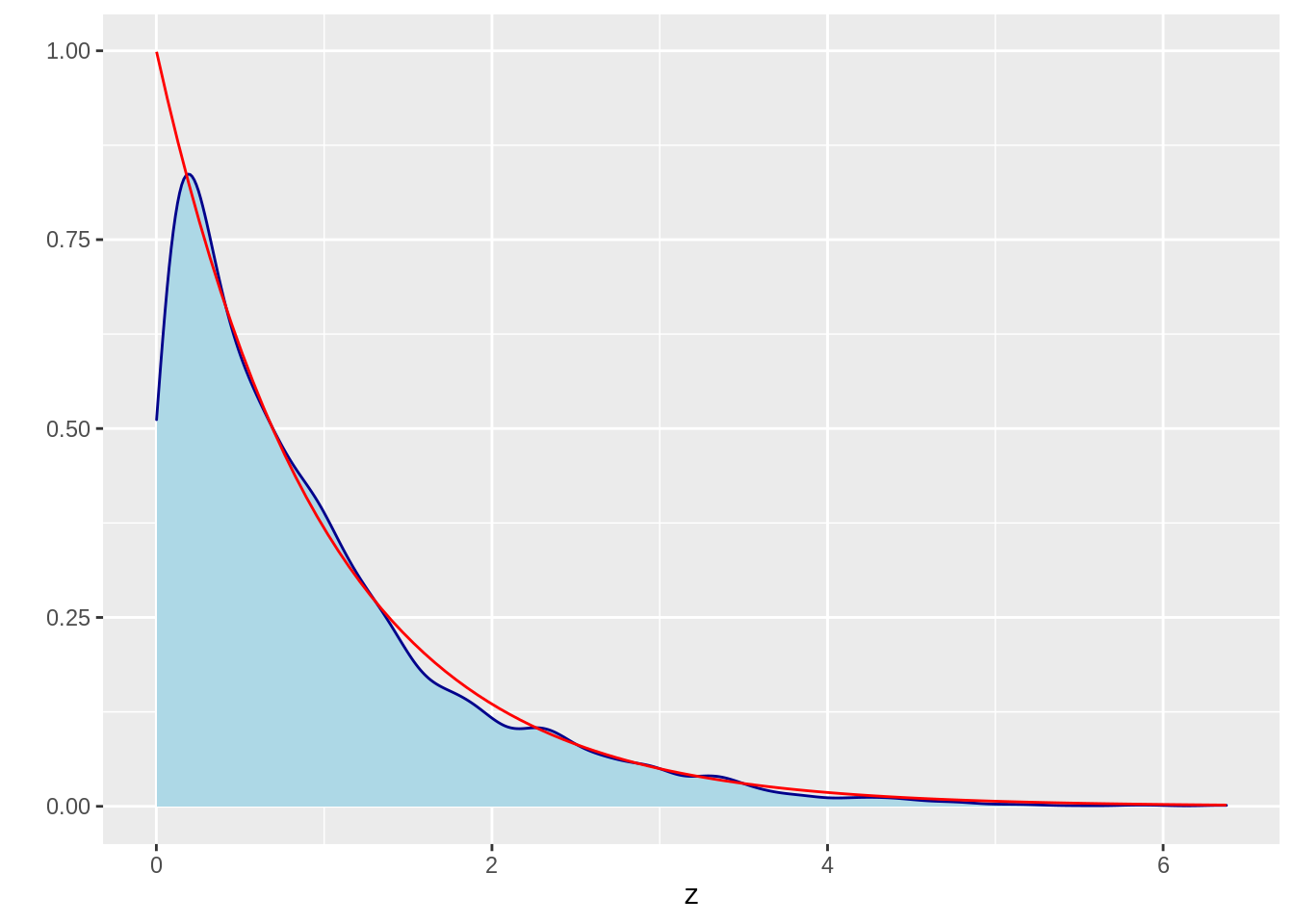
52.7.1 1. Sampling from an exponential distribution
52.7.1.1 a) Define the pdf of exponential distribution
52.7.1.2 b) Define the MCMC function
52.7.2 2. Sampling from a normal distribution
52.7.2.2 b) use previous function and validate the result
z = MCMC(5000,3, 1, norm_dist)
z = data.frame(z)
ggplot(data=z,aes(x=z)) +
  geom_density(color="darkblue", fill="lightblue") +
  stat_function(fun = dnorm, colour = "red") +
  ylab("")
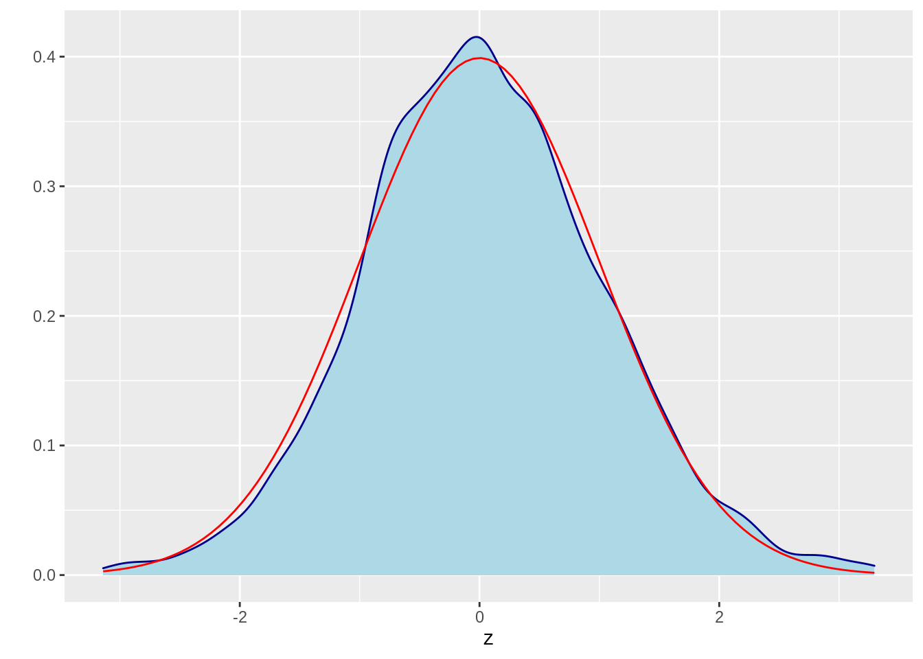
Again, we find the density function is similar to the true distribution.
52.8 8 Refenence
https://en.wikipedia.org/wiki/Markov_chain_Monte_Carlo
http://www.yaroslavvb.com/papers/peres-markov.pdf
https://www.cnblogs.com/pinard/p/6638955.html
https://blog.csdn.net/weixin_30745553/article/details/98648799
https://github.com/ljpzzz/machinelearning/blob/master/mathematics
https://stephens999.github.io/fiveMinuteStats/MH-examples1.html
