Chapter 51 Laying out multiple plots for Baseplot and ggplot
Zhiyi Chen (zc2489)
51.1 Overview
In the process of data analysis, single plot showing is likely to be a weak visual shock. Instead, sometimes several plots should be output which are used for comparison or more strong evidence to verify our ideas. How to lay out several plots seems to be a easy stuff, however, type of plotting, the scale of different plots and other details will make laying out multiple plots in one page difficult. In this tutorial, I will introduce some method from easy use to comprehensive use and pinpoint matters need attention to make the visualizaton logically and readable.
51.2 Most easy and normal form par()
| Parameter | value |
|---|---|
| … | In the form: Tag = value |
| no.readonly | TRUE/FALSE |
More Tag = value can be seen from this link: https://www.rdocumentation.org/packages/graphics/versions/3.6.2/topics/par
par() is a function to create a whole setting for plots. ... shows we can set parameters in form Tag = value, we take no.readonly is equal to TRUE when there is no input in ..., which means it will shows the previous par() settings. Of course, layout of multiple plots can be constructed within par(). The mfrow and mfcol parameters allow us to create a matrix of plots in one plotting space. Both parameters take a vector of length two as an argument, corresponding to the number of rows and columns in the resulting plotting matrix. For example, the following code sets up a 2 x 2 plotting matrix. The difference between mfrow and mfcol is that the former one is by row and the latter one is by column.
# store the previous plot settings
opar <- par(no.readonly = TRUE)

# set 2 x 2 layout
par(mfrow = c(2,2))

# First plot: line chart
plot(c(7,12,28,3,41), type = 'o')

#  Second plot: scatter plot
plot(iris$Sepal.Length, iris$Sepal.Width, main = 'scatter plot', xlab = 'Sepal length', ylab = 'Sepal width')

# Third plot: histgram chart
hist(iris$Sepal.Length, main = 'Histgram chart', xlab = 'Sepal length')

# Fourth plot: boxplot
boxplot(Petal.Length ~ Species, data = iris)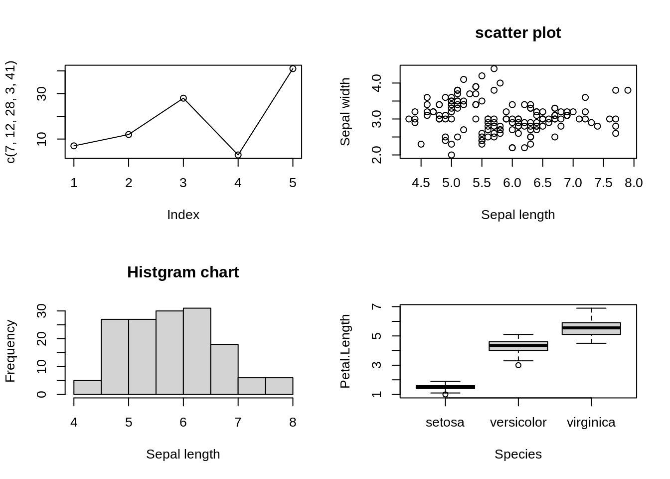
There is one thing need attention that from then on, all the layout will be 2x2 since par() is set for all plots. Otherwise we reset par() or recall the setting before par()
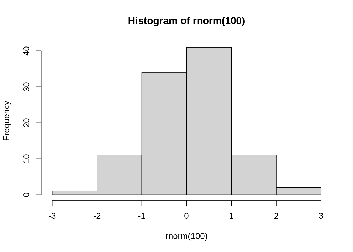
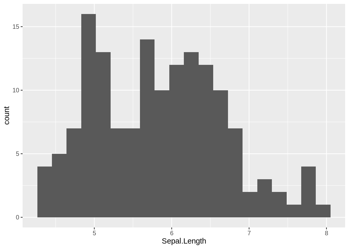
One disadvantage for par() is that it cannot work for ggplot, we can see below that the plot should appear on the upper left of the page, but it just happen as if par() isn’t written here. However, don’t worry about it since ggplot has another function to lay out which is very similar to par() and we will discuss about it later.
51.3 Complex plot layouts with layout()
| Parameter | value |
|---|---|
| mat | a matrix object specifying the location of the next figures on the output device. |
| widths | a vector of values for the widths of columns on the device. |
| heights | a vector of values for the heights of rows on the device. |
| respect | controls whether a unit column-width is the same physical measurement on the device as a unit row-height. |
layout is not a plotting parameter, rather it is a function all on its own. Different from par(), layout() can align position number to certain plot and define the width and height of plot area respectively. We can first have a look to understand how it works.
layout.matrix <- matrix(c(2, 1, 0, 3), nrow = 2, ncol = 2)

layout(mat = layout.matrix,
       heights = c(1, 2), # Heights of the two rows
       widths = c(2, 2)) # Widths of the two columns

layout.show(3)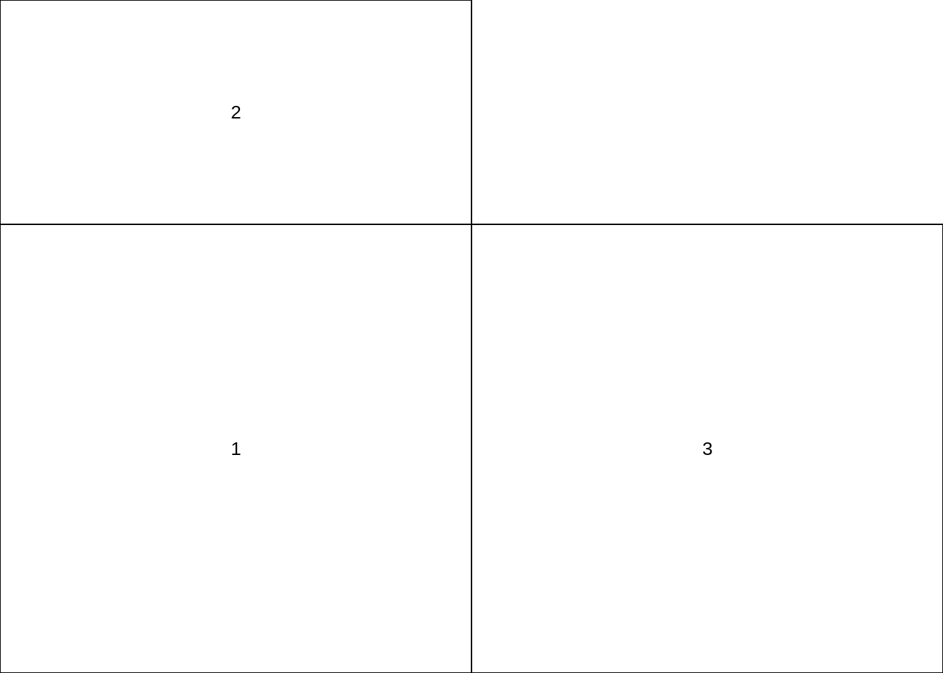
From above chart, 0 means there will be an empty area, 1-3 means the order of plot query, heights here means the length of second row will be 2 times the first row, widths means the length of first column and second column is the same. Moreover, heights and widths will use the same scale. Let use an example to show how layout() performs.
The example is from : https://www.rdocumentation.org/packages/graphics/versions/3.6.2/topics/layout
# Get the data manually
x <- pmin(3, pmax(-3, stats::rnorm(50)))
y <- pmin(3, pmax(-3, stats::rnorm(50)))
xhist <- hist(x, breaks = seq(-3,3,0.5), plot = FALSE)
yhist <- hist(y, breaks = seq(-3,3,0.5), plot = FALSE)
top <- max(c(xhist$counts, yhist$counts))
xrange <- c(-3, 3)
yrange <- c(-3, 3)

# Create a multiple plot layout interface
nf <- layout(matrix(c(2,0,1,3),2,2,byrow = TRUE), c(3,1), c(1,3), TRUE)

# plot 1
par(mar = c(3,3,1,1))           # mar = c(down, left, up, right)
plot(x, y, xlim = xrange, ylim = yrange, xlab = "", ylab = "")

# plot 2
par(mar = c(0,3,1,1))
barplot(xhist$counts, axes = FALSE, ylim = c(0, top), space = 0)

# plot 3
par(mar = c(3,0,1,1))
barplot(yhist$counts, axes = FALSE, xlim = c(0, top), space = 0, horiz = TRUE)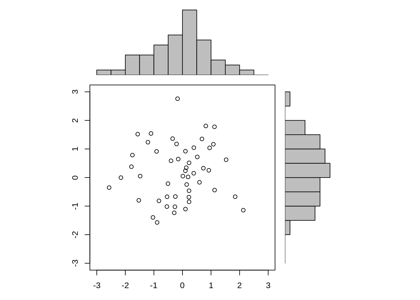
In this case, it is obvious to see the density distribution from two variables and also scatter plot can be seen which gives our a direct and reliable visual shock. It is no doubt that layout() is able to let us better understand data.
51.4 Layout for ggplot
51.4.1 grid.arrange() in gridExtra
| Parameter | value |
|---|---|
| … | grobs, gtables, ggplot or trellis objects |
| grobs | list of grobs(graphical object) |
| layout_matrix | structure of layout |
| widths | c() |
| heights | c() |
| ncol | the number of columns |
| nrow | the number of rows |
More parameter description can be found: https://www.rdocumentation.org/packages/gridExtra/versions/2.3/topics/arrangeGrob
grid.arrange is able to work for grobs, gtables, ggplots, the function and strategy is very similar to par(). ... means the plots we need to combine on a single page. widths,heights,ncol and nrow are the parameters we are very familiar with. Here we still use an example to show how it works.
# prepare all ggplots
p1 <- qplot(Sepal.Length,Sepal.Width,data = iris,col=Species)
p2 <- qplot(Petal.Length, data = iris, binwidth = 0.1) + ggtitle("Histogram")
p3 <- ggplot(data = iris, aes(x = Species, y = Petal.Length)) + geom_boxplot()
p4 <- ggplot(data = iris, aes(x = Sepal.Length, y = Sepal.Width)) + geom_point(aes(col = Species)) +
      facet_wrap( ~ Species, nrow = 1) + theme(legend.position = "none") +
      ggtitle("facetted plot")

# use grid.arrange()
grid.arrange(p1,p2,p3,p4,nrow = 2, widths = c(1,1.5))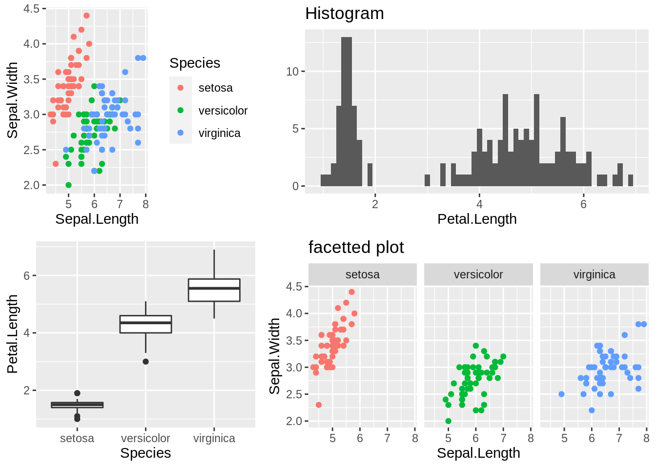
51.4.2 method in grid
The functions in grid also can be used for arranging plots and it is easy for us to align postion for certain graph. One thing worth attention is that we have to write grid.newpage() first to record all the graphs below. I use the example which is one of first questions in homework 3 to display the layout work.
# plots
pr <- data.frame(penguins_raw)
g1 <- ggparcoord(pr, columns = c(10,11,12,13,15,16),alphaLines = 0.3, groupColumn = "Species") + ggtitle("Clusters in Species")
g2 <- ggparcoord(pr, columns = c(10,11,12,13,15,16),alphaLines = 0.3, groupColumn = "Island") + ggtitle("Clusters in Island")
g3 <- ggparcoord(pr, columns = c(10,11,12,13,15,16),alphaLines = 0.3, groupColumn = "Clutch.Completion") + ggtitle("clusters in Clutch.Completion")
g4 <- ggparcoord(pr, columns = c(10,11,12,13,15,16),alphaLines = 0.3, groupColumn = "Date.Egg") + ggtitle("Clusters in Date.Egg")
g5 <- ggparcoord(pr, columns = c(10,11,12,13,15,16),alphaLines = 0.3, groupColumn = "Sex")

# the function in grid to arrange the plots
grid.newpage()
pushViewport(viewport(layout = grid.layout(3, 2)))
vplayout <- function(x, y) viewport(layout.pos.row = x, layout.pos.col = y)
print(g1, vp = vplayout(1, 1:2))
print(g2, vp = vplayout(2, 1))
print(g3, vp = vplayout(2, 2))
print(g4, vp = vplayout(3, 1))
print(g5, vp = vplayout(3, 2))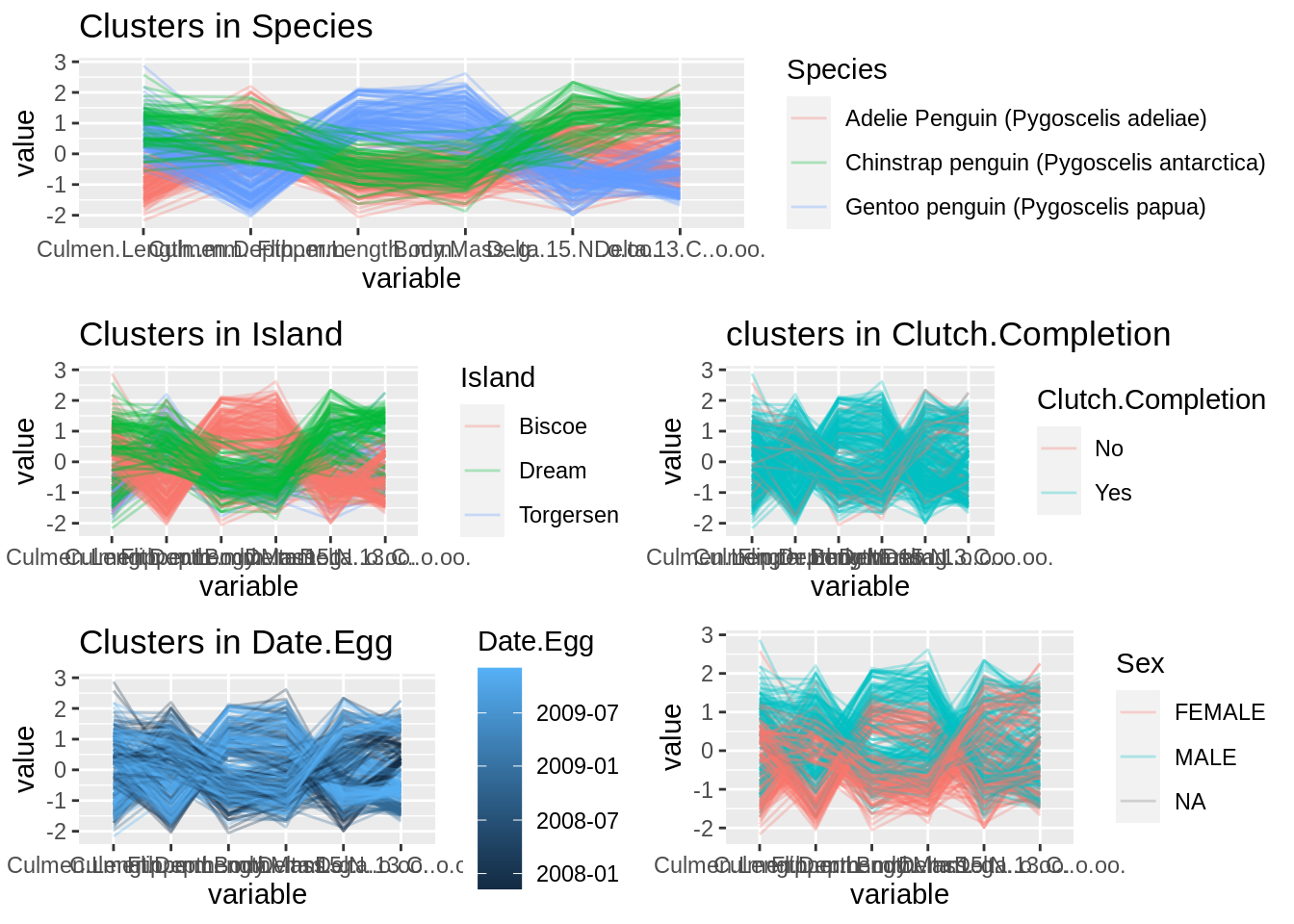
51.5 Reference
More about par() and layout(): https://bookdown.org/ndphillips/YaRrr/arranging-plots-with-parmfrow-and-layout.html
More about layout for ggplot: https://cran.r-project.org/web/packages/egg/vignettes/Ecosystem.html
More about custom layout: https://blog.csdn.net/kMD8d5R/article/details/85182184 (Chinese version)