Chapter 3 Data transformation in R
Jiongxin Ye and Zhuoyan Ma
3.1 Introduction
Data visualizations are nice and insightful, but we usually spend more time formatting, cleaning and wrangling the data. Sometimes, we need to transform the data to perform a better visualization, or maybe we just want to rename the variables and get summaries. No matter for detect factual information or implicit relationships, data transformation plays an important role, helping us to dig deeper and wider and thus telling a better story from data.
As a result, we want share some useful methods of data transformation to let you play with data more efficiently. Specifically, we want to provide a detailed instruction of package dplyr. We hope that you can know the various methods in changing the data frame and function in selecting the data which you want after reading this article.
3.2 Basics
As said before, we will mainly use dplyr package, which will be automatically installed if you install the tidyverse.
- filter: select observations by their values
- arrange: reorder observations
- select: pick variables by their names
- mutate: create or rename variables
- summarize: aggregate observations
- group_by: group observations by variables
All dplyr “verbs” are functions that take a data frame and return a data frame after the operation
To explore the basic data manipulation of dplur, we will demonstrate using nycflights13::flights. It’s a dataset which contains information of 336,776 flights that departed from New York City in 2013. You can access it by installing the packages ‘nycflights13’.
## [90m# A tibble: 336,776 x 19[39m
## year month day dep_time sched_dep_time dep_delay arr_time sched_arr_time
## [3m[90m<int>[39m[23m [3m[90m<int>[39m[23m [3m[90m<int>[39m[23m [3m[90m<int>[39m[23m [3m[90m<int>[39m[23m [3m[90m<dbl>[39m[23m [3m[90m<int>[39m[23m [3m[90m<int>[39m[23m
## [90m 1[39m [4m2[24m013 1 1 517 515 2 830 819
## [90m 2[39m [4m2[24m013 1 1 533 529 4 850 830
## [90m 3[39m [4m2[24m013 1 1 542 540 2 923 850
## [90m 4[39m [4m2[24m013 1 1 544 545 -[31m1[39m [4m1[24m004 [4m1[24m022
## [90m 5[39m [4m2[24m013 1 1 554 600 -[31m6[39m 812 837
## [90m 6[39m [4m2[24m013 1 1 554 558 -[31m4[39m 740 728
## [90m 7[39m [4m2[24m013 1 1 555 600 -[31m5[39m 913 854
## [90m 8[39m [4m2[24m013 1 1 557 600 -[31m3[39m 709 723
## [90m 9[39m [4m2[24m013 1 1 557 600 -[31m3[39m 838 846
## [90m10[39m [4m2[24m013 1 1 558 600 -[31m2[39m 753 745
## [90m# … with 336,766 more rows, and 11 more variables: arr_delay [3m[90m<dbl>[90m[23m,[39m
## [90m# carrier [3m[90m<chr>[90m[23m, flight [3m[90m<int>[90m[23m, tailnum [3m[90m<chr>[90m[23m, origin [3m[90m<chr>[90m[23m, dest [3m[90m<chr>[90m[23m,[39m
## [90m# air_time [3m[90m<dbl>[90m[23m, distance [3m[90m<dbl>[90m[23m, hour [3m[90m<dbl>[90m[23m, minute [3m[90m<dbl>[90m[23m, time_hour [3m[90m<dttm>[90m[23m[39m3.3 Function Usage
3.3.1 1. Filter( )
To select observations we can use filter:
filter (.data, condition1, condition2, …, conditionN)
where each condition evaluates to a logical vector and only TRUE entries are kept.
Example:
- we want to focus on the flight whose carrier is UA.
## [90m# A tibble: 6 x 19[39m
## year month day dep_time sched_dep_time dep_delay arr_time sched_arr_time
## [3m[90m<int>[39m[23m [3m[90m<int>[39m[23m [3m[90m<int>[39m[23m [3m[90m<int>[39m[23m [3m[90m<int>[39m[23m [3m[90m<dbl>[39m[23m [3m[90m<int>[39m[23m [3m[90m<int>[39m[23m
## [90m1[39m [4m2[24m013 1 1 517 515 2 830 819
## [90m2[39m [4m2[24m013 1 1 533 529 4 850 830
## [90m3[39m [4m2[24m013 1 1 554 558 -[31m4[39m 740 728
## [90m4[39m [4m2[24m013 1 1 558 600 -[31m2[39m 924 917
## [90m5[39m [4m2[24m013 1 1 558 600 -[31m2[39m 923 937
## [90m6[39m [4m2[24m013 1 1 559 600 -[31m1[39m 854 902
## [90m# … with 11 more variables: arr_delay [3m[90m<dbl>[90m[23m, carrier [3m[90m<chr>[90m[23m, flight [3m[90m<int>[90m[23m,[39m
## [90m# tailnum [3m[90m<chr>[90m[23m, origin [3m[90m<chr>[90m[23m, dest [3m[90m<chr>[90m[23m, air_time [3m[90m<dbl>[90m[23m, distance [3m[90m<dbl>[90m[23m,[39m
## [90m# hour [3m[90m<dbl>[90m[23m, minute [3m[90m<dbl>[90m[23m, time_hour [3m[90m<dttm>[90m[23m[39mWhat we found:
There are UA_num, 58665, flights whose carrier is UA in nycflights13 dataset.
- We also can use filter to remove rows that associated with NA values of certain variables like dep_time.
What we found:
we remove over 8,000 rows whose dep_time is NA. The total number of observations after removing the NA objects in dep_time is dep_num, which is 328521.
- More importantly, we can cooperate with logical operators ! (not), | (or), & (and) and some statistical rules such as De Morgan’s Law, to add more conditions in the filter function in a way you like.
Below three approaches are equivalent to find flights in January and Feburary.
## [90m# A tibble: 51,955 x 19[39m
## year month day dep_time sched_dep_time dep_delay arr_time sched_arr_time
## [3m[90m<int>[39m[23m [3m[90m<int>[39m[23m [3m[90m<int>[39m[23m [3m[90m<int>[39m[23m [3m[90m<int>[39m[23m [3m[90m<dbl>[39m[23m [3m[90m<int>[39m[23m [3m[90m<int>[39m[23m
## [90m 1[39m [4m2[24m013 1 1 517 515 2 830 819
## [90m 2[39m [4m2[24m013 1 1 533 529 4 850 830
## [90m 3[39m [4m2[24m013 1 1 542 540 2 923 850
## [90m 4[39m [4m2[24m013 1 1 544 545 -[31m1[39m [4m1[24m004 [4m1[24m022
## [90m 5[39m [4m2[24m013 1 1 554 600 -[31m6[39m 812 837
## [90m 6[39m [4m2[24m013 1 1 554 558 -[31m4[39m 740 728
## [90m 7[39m [4m2[24m013 1 1 555 600 -[31m5[39m 913 854
## [90m 8[39m [4m2[24m013 1 1 557 600 -[31m3[39m 709 723
## [90m 9[39m [4m2[24m013 1 1 557 600 -[31m3[39m 838 846
## [90m10[39m [4m2[24m013 1 1 558 600 -[31m2[39m 753 745
## [90m# … with 51,945 more rows, and 11 more variables: arr_delay [3m[90m<dbl>[90m[23m,[39m
## [90m# carrier [3m[90m<chr>[90m[23m, flight [3m[90m<int>[90m[23m, tailnum [3m[90m<chr>[90m[23m, origin [3m[90m<chr>[90m[23m, dest [3m[90m<chr>[90m[23m,[39m
## [90m# air_time [3m[90m<dbl>[90m[23m, distance [3m[90m<dbl>[90m[23m, hour [3m[90m<dbl>[90m[23m, minute [3m[90m<dbl>[90m[23m, time_hour [3m[90m<dttm>[90m[23m[39m## [90m# A tibble: 51,955 x 19[39m
## year month day dep_time sched_dep_time dep_delay arr_time sched_arr_time
## [3m[90m<int>[39m[23m [3m[90m<int>[39m[23m [3m[90m<int>[39m[23m [3m[90m<int>[39m[23m [3m[90m<int>[39m[23m [3m[90m<dbl>[39m[23m [3m[90m<int>[39m[23m [3m[90m<int>[39m[23m
## [90m 1[39m [4m2[24m013 1 1 517 515 2 830 819
## [90m 2[39m [4m2[24m013 1 1 533 529 4 850 830
## [90m 3[39m [4m2[24m013 1 1 542 540 2 923 850
## [90m 4[39m [4m2[24m013 1 1 544 545 -[31m1[39m [4m1[24m004 [4m1[24m022
## [90m 5[39m [4m2[24m013 1 1 554 600 -[31m6[39m 812 837
## [90m 6[39m [4m2[24m013 1 1 554 558 -[31m4[39m 740 728
## [90m 7[39m [4m2[24m013 1 1 555 600 -[31m5[39m 913 854
## [90m 8[39m [4m2[24m013 1 1 557 600 -[31m3[39m 709 723
## [90m 9[39m [4m2[24m013 1 1 557 600 -[31m3[39m 838 846
## [90m10[39m [4m2[24m013 1 1 558 600 -[31m2[39m 753 745
## [90m# … with 51,945 more rows, and 11 more variables: arr_delay [3m[90m<dbl>[90m[23m,[39m
## [90m# carrier [3m[90m<chr>[90m[23m, flight [3m[90m<int>[90m[23m, tailnum [3m[90m<chr>[90m[23m, origin [3m[90m<chr>[90m[23m, dest [3m[90m<chr>[90m[23m,[39m
## [90m# air_time [3m[90m<dbl>[90m[23m, distance [3m[90m<dbl>[90m[23m, hour [3m[90m<dbl>[90m[23m, minute [3m[90m<dbl>[90m[23m, time_hour [3m[90m<dttm>[90m[23m[39m3.3.1.1 More exercises:
Find flights that:
- Were delayed by at least an hour, but made up over 30 minutes in flight
## [90m# A tibble: 2,046 x 19[39m
## year month day dep_time sched_dep_time dep_delay arr_time sched_arr_time
## [3m[90m<int>[39m[23m [3m[90m<int>[39m[23m [3m[90m<int>[39m[23m [3m[90m<int>[39m[23m [3m[90m<int>[39m[23m [3m[90m<dbl>[39m[23m [3m[90m<int>[39m[23m [3m[90m<int>[39m[23m
## [90m 1[39m [4m2[24m013 1 1 [4m1[24m716 [4m1[24m545 91 [4m2[24m140 [4m2[24m039
## [90m 2[39m [4m2[24m013 1 1 [4m2[24m205 [4m1[24m720 285 46 [4m2[24m040
## [90m 3[39m [4m2[24m013 1 1 [4m2[24m326 [4m2[24m130 116 131 18
## [90m 4[39m [4m2[24m013 1 3 [4m1[24m503 [4m1[24m221 162 [4m1[24m803 [4m1[24m555
## [90m 5[39m [4m2[24m013 1 3 [4m1[24m821 [4m1[24m530 171 [4m2[24m131 [4m1[24m910
## [90m 6[39m [4m2[24m013 1 3 [4m1[24m839 [4m1[24m700 99 [4m2[24m056 [4m1[24m950
## [90m 7[39m [4m2[24m013 1 3 [4m1[24m850 [4m1[24m745 65 [4m2[24m148 [4m2[24m120
## [90m 8[39m [4m2[24m013 1 3 [4m1[24m923 [4m1[24m815 68 [4m2[24m036 [4m1[24m958
## [90m 9[39m [4m2[24m013 1 3 [4m1[24m941 [4m1[24m759 102 [4m2[24m246 [4m2[24m139
## [90m10[39m [4m2[24m013 1 3 [4m1[24m950 [4m1[24m845 65 [4m2[24m228 [4m2[24m227
## [90m# … with 2,036 more rows, and 11 more variables: arr_delay [3m[90m<dbl>[90m[23m,[39m
## [90m# carrier [3m[90m<chr>[90m[23m, flight [3m[90m<int>[90m[23m, tailnum [3m[90m<chr>[90m[23m, origin [3m[90m<chr>[90m[23m, dest [3m[90m<chr>[90m[23m,[39m
## [90m# air_time [3m[90m<dbl>[90m[23m, distance [3m[90m<dbl>[90m[23m, hour [3m[90m<dbl>[90m[23m, minute [3m[90m<dbl>[90m[23m, time_hour [3m[90m<dttm>[90m[23m[39m- Flew to Boston operated by United, American or Delta in Summer (June to August)
filter(flights, dest == "BOS",
carrier == "UA" | carrier == "AA" | carrier == "DL",
month %in% c(6, 7, 8))
## [90m# A tibble: 1,663 x 19[39m
## year month day dep_time sched_dep_time dep_delay arr_time sched_arr_time
## [3m[90m<int>[39m[23m [3m[90m<int>[39m[23m [3m[90m<int>[39m[23m [3m[90m<int>[39m[23m [3m[90m<int>[39m[23m [3m[90m<dbl>[39m[23m [3m[90m<int>[39m[23m [3m[90m<int>[39m[23m
## [90m 1[39m [4m2[24m013 6 1 816 820 -[31m4[39m 920 930
## [90m 2[39m [4m2[24m013 6 1 [4m1[24m022 [4m1[24m025 -[31m3[39m [4m1[24m130 [4m1[24m150
## [90m 3[39m [4m2[24m013 6 1 [4m1[24m240 [4m1[24m245 -[31m5[39m [4m1[24m343 [4m1[24m350
## [90m 4[39m [4m2[24m013 6 1 [4m1[24m519 [4m1[24m530 -[31m11[39m [4m1[24m705 [4m1[24m702
## [90m 5[39m [4m2[24m013 6 1 [4m1[24m524 [4m1[24m445 39 [4m1[24m634 [4m1[24m615
## [90m 6[39m [4m2[24m013 6 1 [4m1[24m555 [4m1[24m600 -[31m5[39m [4m1[24m705 [4m1[24m720
## [90m 7[39m [4m2[24m013 6 1 [4m1[24m954 [4m1[24m955 -[31m1[39m [4m2[24m116 [4m2[24m110
## [90m 8[39m [4m2[24m013 6 1 [4m2[24m010 [4m2[24m000 10 [4m2[24m115 [4m2[24m130
## [90m 9[39m [4m2[24m013 6 1 [4m2[24m124 [4m2[24m125 -[31m1[39m [4m2[24m224 [4m2[24m256
## [90m10[39m [4m2[24m013 6 1 [4m2[24m152 [4m2[24m159 -[31m7[39m [4m2[24m252 [4m2[24m328
## [90m# … with 1,653 more rows, and 11 more variables: arr_delay [3m[90m<dbl>[90m[23m,[39m
## [90m# carrier [3m[90m<chr>[90m[23m, flight [3m[90m<int>[90m[23m, tailnum [3m[90m<chr>[90m[23m, origin [3m[90m<chr>[90m[23m, dest [3m[90m<chr>[90m[23m,[39m
## [90m# air_time [3m[90m<dbl>[90m[23m, distance [3m[90m<dbl>[90m[23m, hour [3m[90m<dbl>[90m[23m, minute [3m[90m<dbl>[90m[23m, time_hour [3m[90m<dttm>[90m[23m[39m3.3.2 2. Arrange( )
Arrange( ) function lets us to reorder the rows in a order that we want:
arrange (.data, variable1, variable2,…, .by_group = FALSE)
It’s default in increasing order. To reorder decreasingly, use desc. You can also reorder the rows by group, using .by_group.
Example:
- we can reorder the flight by the delay in departure in a increasing order.
## [90m# A tibble: 336,776 x 19[39m
## year month day dep_time sched_dep_time dep_delay arr_time sched_arr_time
## [3m[90m<int>[39m[23m [3m[90m<int>[39m[23m [3m[90m<int>[39m[23m [3m[90m<int>[39m[23m [3m[90m<int>[39m[23m [3m[90m<dbl>[39m[23m [3m[90m<int>[39m[23m [3m[90m<int>[39m[23m
## [90m 1[39m [4m2[24m013 12 7 [4m2[24m040 [4m2[24m123 -[31m43[39m 40 [4m2[24m352
## [90m 2[39m [4m2[24m013 2 3 [4m2[24m022 [4m2[24m055 -[31m33[39m [4m2[24m240 [4m2[24m338
## [90m 3[39m [4m2[24m013 11 10 [4m1[24m408 [4m1[24m440 -[31m32[39m [4m1[24m549 [4m1[24m559
## [90m 4[39m [4m2[24m013 1 11 [4m1[24m900 [4m1[24m930 -[31m30[39m [4m2[24m233 [4m2[24m243
## [90m 5[39m [4m2[24m013 1 29 [4m1[24m703 [4m1[24m730 -[31m27[39m [4m1[24m947 [4m1[24m957
## [90m 6[39m [4m2[24m013 8 9 729 755 -[31m26[39m [4m1[24m002 955
## [90m 7[39m [4m2[24m013 10 23 [4m1[24m907 [4m1[24m932 -[31m25[39m [4m2[24m143 [4m2[24m143
## [90m 8[39m [4m2[24m013 3 30 [4m2[24m030 [4m2[24m055 -[31m25[39m [4m2[24m213 [4m2[24m250
## [90m 9[39m [4m2[24m013 3 2 [4m1[24m431 [4m1[24m455 -[31m24[39m [4m1[24m601 [4m1[24m631
## [90m10[39m [4m2[24m013 5 5 934 958 -[31m24[39m [4m1[24m225 [4m1[24m309
## [90m# … with 336,766 more rows, and 11 more variables: arr_delay [3m[90m<dbl>[90m[23m,[39m
## [90m# carrier [3m[90m<chr>[90m[23m, flight [3m[90m<int>[90m[23m, tailnum [3m[90m<chr>[90m[23m, origin [3m[90m<chr>[90m[23m, dest [3m[90m<chr>[90m[23m,[39m
## [90m# air_time [3m[90m<dbl>[90m[23m, distance [3m[90m<dbl>[90m[23m, hour [3m[90m<dbl>[90m[23m, minute [3m[90m<dbl>[90m[23m, time_hour [3m[90m<dttm>[90m[23m[39mWhat we found:
The data has been reorder by dep_delay value from small to large.
- we can reorder the flight by the delay in departure in a decreasing order.
## [90m# A tibble: 336,776 x 19[39m
## year month day dep_time sched_dep_time dep_delay arr_time sched_arr_time
## [3m[90m<int>[39m[23m [3m[90m<int>[39m[23m [3m[90m<int>[39m[23m [3m[90m<int>[39m[23m [3m[90m<int>[39m[23m [3m[90m<dbl>[39m[23m [3m[90m<int>[39m[23m [3m[90m<int>[39m[23m
## [90m 1[39m [4m2[24m013 1 9 641 900 [4m1[24m301 [4m1[24m242 [4m1[24m530
## [90m 2[39m [4m2[24m013 6 15 [4m1[24m432 [4m1[24m935 [4m1[24m137 [4m1[24m607 [4m2[24m120
## [90m 3[39m [4m2[24m013 1 10 [4m1[24m121 [4m1[24m635 [4m1[24m126 [4m1[24m239 [4m1[24m810
## [90m 4[39m [4m2[24m013 9 20 [4m1[24m139 [4m1[24m845 [4m1[24m014 [4m1[24m457 [4m2[24m210
## [90m 5[39m [4m2[24m013 7 22 845 [4m1[24m600 [4m1[24m005 [4m1[24m044 [4m1[24m815
## [90m 6[39m [4m2[24m013 4 10 [4m1[24m100 [4m1[24m900 960 [4m1[24m342 [4m2[24m211
## [90m 7[39m [4m2[24m013 3 17 [4m2[24m321 810 911 135 [4m1[24m020
## [90m 8[39m [4m2[24m013 6 27 959 [4m1[24m900 899 [4m1[24m236 [4m2[24m226
## [90m 9[39m [4m2[24m013 7 22 [4m2[24m257 759 898 121 [4m1[24m026
## [90m10[39m [4m2[24m013 12 5 756 [4m1[24m700 896 [4m1[24m058 [4m2[24m020
## [90m# … with 336,766 more rows, and 11 more variables: arr_delay [3m[90m<dbl>[90m[23m,[39m
## [90m# carrier [3m[90m<chr>[90m[23m, flight [3m[90m<int>[90m[23m, tailnum [3m[90m<chr>[90m[23m, origin [3m[90m<chr>[90m[23m, dest [3m[90m<chr>[90m[23m,[39m
## [90m# air_time [3m[90m<dbl>[90m[23m, distance [3m[90m<dbl>[90m[23m, hour [3m[90m<dbl>[90m[23m, minute [3m[90m<dbl>[90m[23m, time_hour [3m[90m<dttm>[90m[23m[39mWhat we found:
The data has been reorder by dep_delay value from large to small.
- we can reorder the flight by the month and day.
## [90m# A tibble: 336,776 x 19[39m
## year month day dep_time sched_dep_time dep_delay arr_time sched_arr_time
## [3m[90m<int>[39m[23m [3m[90m<int>[39m[23m [3m[90m<int>[39m[23m [3m[90m<int>[39m[23m [3m[90m<int>[39m[23m [3m[90m<dbl>[39m[23m [3m[90m<int>[39m[23m [3m[90m<int>[39m[23m
## [90m 1[39m [4m2[24m013 1 1 517 515 2 830 819
## [90m 2[39m [4m2[24m013 1 1 533 529 4 850 830
## [90m 3[39m [4m2[24m013 1 1 542 540 2 923 850
## [90m 4[39m [4m2[24m013 1 1 544 545 -[31m1[39m [4m1[24m004 [4m1[24m022
## [90m 5[39m [4m2[24m013 1 1 554 600 -[31m6[39m 812 837
## [90m 6[39m [4m2[24m013 1 1 554 558 -[31m4[39m 740 728
## [90m 7[39m [4m2[24m013 1 1 555 600 -[31m5[39m 913 854
## [90m 8[39m [4m2[24m013 1 1 557 600 -[31m3[39m 709 723
## [90m 9[39m [4m2[24m013 1 1 557 600 -[31m3[39m 838 846
## [90m10[39m [4m2[24m013 1 1 558 600 -[31m2[39m 753 745
## [90m# … with 336,766 more rows, and 11 more variables: arr_delay [3m[90m<dbl>[90m[23m,[39m
## [90m# carrier [3m[90m<chr>[90m[23m, flight [3m[90m<int>[90m[23m, tailnum [3m[90m<chr>[90m[23m, origin [3m[90m<chr>[90m[23m, dest [3m[90m<chr>[90m[23m,[39m
## [90m# air_time [3m[90m<dbl>[90m[23m, distance [3m[90m<dbl>[90m[23m, hour [3m[90m<dbl>[90m[23m, minute [3m[90m<dbl>[90m[23m, time_hour [3m[90m<dttm>[90m[23m[39mWhat we found:
The data has been reorder by 2 variables: month and day. For the object with same month, they are reordering by day.
- we can reorder the flight by the delay in departure in a decreasing order group by carrier.
## [90m# A tibble: 336,776 x 19[39m
## [90m# Groups: carrier [16][39m
## year month day dep_time sched_dep_time dep_delay arr_time sched_arr_time
## [3m[90m<int>[39m[23m [3m[90m<int>[39m[23m [3m[90m<int>[39m[23m [3m[90m<int>[39m[23m [3m[90m<int>[39m[23m [3m[90m<dbl>[39m[23m [3m[90m<int>[39m[23m [3m[90m<int>[39m[23m
## [90m 1[39m [4m2[24m013 2 16 757 [4m1[24m930 747 [4m1[24m013 [4m2[24m149
## [90m 2[39m [4m2[24m013 7 24 [4m1[24m525 815 430 [4m1[24m808 [4m1[24m030
## [90m 3[39m [4m2[24m013 11 27 [4m1[24m503 815 408 [4m1[24m628 952
## [90m 4[39m [4m2[24m013 2 27 [4m1[24m529 845 404 [4m1[24m639 [4m1[24m015
## [90m 5[39m [4m2[24m013 7 7 [4m2[24m228 [4m1[24m559 389 [31mNA[39m [4m1[24m828
## [90m 6[39m [4m2[24m013 6 25 [4m1[24m421 805 376 [4m1[24m602 950
## [90m 7[39m [4m2[24m013 1 25 15 [4m1[24m815 360 208 [4m1[24m958
## [90m 8[39m [4m2[24m013 12 14 [4m1[24m425 825 360 [4m1[24m604 938
## [90m 9[39m [4m2[24m013 9 12 [4m2[24m159 [4m1[24m600 359 [4m2[24m400 [4m1[24m818
## [90m10[39m [4m2[24m013 7 22 [4m2[24m216 [4m1[24m620 356 116 [4m1[24m853
## [90m# … with 336,766 more rows, and 11 more variables: arr_delay [3m[90m<dbl>[90m[23m,[39m
## [90m# carrier [3m[90m<chr>[90m[23m, flight [3m[90m<int>[90m[23m, tailnum [3m[90m<chr>[90m[23m, origin [3m[90m<chr>[90m[23m, dest [3m[90m<chr>[90m[23m,[39m
## [90m# air_time [3m[90m<dbl>[90m[23m, distance [3m[90m<dbl>[90m[23m, hour [3m[90m<dbl>[90m[23m, minute [3m[90m<dbl>[90m[23m, time_hour [3m[90m<dttm>[90m[23m[39mWhat we found:
The data has been reorder by grouping the carrier and then order by dep_delay value from large to small. Since the carrier is nominal variable, the carrier order is default. Attention: If we don’t use the .by_group in arrange( ), the data will be reorder just by dep_delay value although we have group_by the data in previous.
3.3.3 3. Select( )
It subsets a dataset containing only selected variables.
select (.data, variable_expression)
Some helper functions:
- Negative indices remove variables from the selection.
- A:B, from column A to column B
- starts_with(“abc”): matches names starting with “abc”
- ends_with(“xyz”): matches names ending with “xyz”
- contains(“ijk”): matches names containing “ijk”
- num_range(“x”, 1:3): matches x1, x2, x3
We can use the operators in selecting the variables easily and use c( ) to combine selections.
Example:
- Select year, month, day, destination columns from flights.
## [90m# A tibble: 336,776 x 4[39m
## year month day dest
## [3m[90m<int>[39m[23m [3m[90m<int>[39m[23m [3m[90m<int>[39m[23m [3m[90m<chr>[39m[23m
## [90m 1[39m [4m2[24m013 1 1 IAH
## [90m 2[39m [4m2[24m013 1 1 IAH
## [90m 3[39m [4m2[24m013 1 1 MIA
## [90m 4[39m [4m2[24m013 1 1 BQN
## [90m 5[39m [4m2[24m013 1 1 ATL
## [90m 6[39m [4m2[24m013 1 1 ORD
## [90m 7[39m [4m2[24m013 1 1 FLL
## [90m 8[39m [4m2[24m013 1 1 IAD
## [90m 9[39m [4m2[24m013 1 1 MCO
## [90m10[39m [4m2[24m013 1 1 ORD
## [90m# … with 336,766 more rows[39mwe can also use the columns number to represent the columns name.
## [90m# A tibble: 336,776 x 4[39m
## year month day dest
## [3m[90m<int>[39m[23m [3m[90m<int>[39m[23m [3m[90m<int>[39m[23m [3m[90m<chr>[39m[23m
## [90m 1[39m [4m2[24m013 1 1 IAH
## [90m 2[39m [4m2[24m013 1 1 IAH
## [90m 3[39m [4m2[24m013 1 1 MIA
## [90m 4[39m [4m2[24m013 1 1 BQN
## [90m 5[39m [4m2[24m013 1 1 ATL
## [90m 6[39m [4m2[24m013 1 1 ORD
## [90m 7[39m [4m2[24m013 1 1 FLL
## [90m 8[39m [4m2[24m013 1 1 IAD
## [90m 9[39m [4m2[24m013 1 1 MCO
## [90m10[39m [4m2[24m013 1 1 ORD
## [90m# … with 336,766 more rows[39mwe can also use | to union the variable set.
## [90m# A tibble: 336,776 x 4[39m
## year month day dest
## [3m[90m<int>[39m[23m [3m[90m<int>[39m[23m [3m[90m<int>[39m[23m [3m[90m<chr>[39m[23m
## [90m 1[39m [4m2[24m013 1 1 IAH
## [90m 2[39m [4m2[24m013 1 1 IAH
## [90m 3[39m [4m2[24m013 1 1 MIA
## [90m 4[39m [4m2[24m013 1 1 BQN
## [90m 5[39m [4m2[24m013 1 1 ATL
## [90m 6[39m [4m2[24m013 1 1 ORD
## [90m 7[39m [4m2[24m013 1 1 FLL
## [90m 8[39m [4m2[24m013 1 1 IAD
## [90m 9[39m [4m2[24m013 1 1 MCO
## [90m10[39m [4m2[24m013 1 1 ORD
## [90m# … with 336,766 more rows[39m- Select all columns except year, month, day, destination from flights.
## [90m# A tibble: 336,776 x 19[39m
## dep_time sched_dep_time dep_delay arr_time sched_arr_time arr_delay carrier
## [3m[90m<int>[39m[23m [3m[90m<int>[39m[23m [3m[90m<dbl>[39m[23m [3m[90m<int>[39m[23m [3m[90m<int>[39m[23m [3m[90m<dbl>[39m[23m [3m[90m<chr>[39m[23m
## [90m 1[39m 517 515 2 830 819 11 UA
## [90m 2[39m 533 529 4 850 830 20 UA
## [90m 3[39m 542 540 2 923 850 33 AA
## [90m 4[39m 544 545 -[31m1[39m [4m1[24m004 [4m1[24m022 -[31m18[39m B6
## [90m 5[39m 554 600 -[31m6[39m 812 837 -[31m25[39m DL
## [90m 6[39m 554 558 -[31m4[39m 740 728 12 UA
## [90m 7[39m 555 600 -[31m5[39m 913 854 19 B6
## [90m 8[39m 557 600 -[31m3[39m 709 723 -[31m14[39m EV
## [90m 9[39m 557 600 -[31m3[39m 838 846 -[31m8[39m B6
## [90m10[39m 558 600 -[31m2[39m 753 745 8 AA
## [90m# … with 336,766 more rows, and 12 more variables: flight [3m[90m<int>[90m[23m, tailnum [3m[90m<chr>[90m[23m,[39m
## [90m# origin [3m[90m<chr>[90m[23m, dest [3m[90m<chr>[90m[23m, air_time [3m[90m<dbl>[90m[23m, distance [3m[90m<dbl>[90m[23m, hour [3m[90m<dbl>[90m[23m,[39m
## [90m# minute [3m[90m<dbl>[90m[23m, time_hour [3m[90m<dttm>[90m[23m, year [3m[90m<int>[90m[23m, month [3m[90m<int>[90m[23m, day [3m[90m<int>[90m[23m[39m- We can also use the c( ) to combine the variables.
## [90m# A tibble: 336,776 x 15[39m
## dep_time sched_dep_time dep_delay arr_time sched_arr_time arr_delay carrier
## [3m[90m<int>[39m[23m [3m[90m<int>[39m[23m [3m[90m<dbl>[39m[23m [3m[90m<int>[39m[23m [3m[90m<int>[39m[23m [3m[90m<dbl>[39m[23m [3m[90m<chr>[39m[23m
## [90m 1[39m 517 515 2 830 819 11 UA
## [90m 2[39m 533 529 4 850 830 20 UA
## [90m 3[39m 542 540 2 923 850 33 AA
## [90m 4[39m 544 545 -[31m1[39m [4m1[24m004 [4m1[24m022 -[31m18[39m B6
## [90m 5[39m 554 600 -[31m6[39m 812 837 -[31m25[39m DL
## [90m 6[39m 554 558 -[31m4[39m 740 728 12 UA
## [90m 7[39m 555 600 -[31m5[39m 913 854 19 B6
## [90m 8[39m 557 600 -[31m3[39m 709 723 -[31m14[39m EV
## [90m 9[39m 557 600 -[31m3[39m 838 846 -[31m8[39m B6
## [90m10[39m 558 600 -[31m2[39m 753 745 8 AA
## [90m# … with 336,766 more rows, and 8 more variables: flight [3m[90m<int>[90m[23m, tailnum [3m[90m<chr>[90m[23m,[39m
## [90m# origin [3m[90m<chr>[90m[23m, air_time [3m[90m<dbl>[90m[23m, distance [3m[90m<dbl>[90m[23m, hour [3m[90m<dbl>[90m[23m, minute [3m[90m<dbl>[90m[23m,[39m
## [90m# time_hour [3m[90m<dttm>[90m[23m[39m- Select columns end with ‘times’.
## [90m# A tibble: 336,776 x 5[39m
## dep_time sched_dep_time arr_time sched_arr_time air_time
## [3m[90m<int>[39m[23m [3m[90m<int>[39m[23m [3m[90m<int>[39m[23m [3m[90m<int>[39m[23m [3m[90m<dbl>[39m[23m
## [90m 1[39m 517 515 830 819 227
## [90m 2[39m 533 529 850 830 227
## [90m 3[39m 542 540 923 850 160
## [90m 4[39m 544 545 [4m1[24m004 [4m1[24m022 183
## [90m 5[39m 554 600 812 837 116
## [90m 6[39m 554 558 740 728 150
## [90m 7[39m 555 600 913 854 158
## [90m 8[39m 557 600 709 723 53
## [90m 9[39m 557 600 838 846 140
## [90m10[39m 558 600 753 745 138
## [90m# … with 336,766 more rows[39m- Select columns end with ‘times’ but without the one starting with ‘sched’.
## [90m# A tibble: 336,776 x 3[39m
## dep_time arr_time air_time
## [3m[90m<int>[39m[23m [3m[90m<int>[39m[23m [3m[90m<dbl>[39m[23m
## [90m 1[39m 517 830 227
## [90m 2[39m 533 850 227
## [90m 3[39m 542 923 160
## [90m 4[39m 544 [4m1[24m004 183
## [90m 5[39m 554 812 116
## [90m 6[39m 554 740 150
## [90m 7[39m 555 913 158
## [90m 8[39m 557 709 53
## [90m 9[39m 557 838 140
## [90m10[39m 558 753 138
## [90m# … with 336,766 more rows[39m- Select columns contains ‘dep’.
## [90m# A tibble: 336,776 x 3[39m
## dep_time sched_dep_time dep_delay
## [3m[90m<int>[39m[23m [3m[90m<int>[39m[23m [3m[90m<dbl>[39m[23m
## [90m 1[39m 517 515 2
## [90m 2[39m 533 529 4
## [90m 3[39m 542 540 2
## [90m 4[39m 544 545 -[31m1[39m
## [90m 5[39m 554 600 -[31m6[39m
## [90m 6[39m 554 558 -[31m4[39m
## [90m 7[39m 555 600 -[31m5[39m
## [90m 8[39m 557 600 -[31m3[39m
## [90m 9[39m 557 600 -[31m3[39m
## [90m10[39m 558 600 -[31m2[39m
## [90m# … with 336,766 more rows[39m- Select year, month, day, destination columns from flights. Also columns end with ‘times’ but without the one starting with ‘sched’.
## [90m# A tibble: 336,776 x 7[39m
## year month day dest dep_time arr_time air_time
## [3m[90m<int>[39m[23m [3m[90m<int>[39m[23m [3m[90m<int>[39m[23m [3m[90m<chr>[39m[23m [3m[90m<int>[39m[23m [3m[90m<int>[39m[23m [3m[90m<dbl>[39m[23m
## [90m 1[39m [4m2[24m013 1 1 IAH 517 830 227
## [90m 2[39m [4m2[24m013 1 1 IAH 533 850 227
## [90m 3[39m [4m2[24m013 1 1 MIA 542 923 160
## [90m 4[39m [4m2[24m013 1 1 BQN 544 [4m1[24m004 183
## [90m 5[39m [4m2[24m013 1 1 ATL 554 812 116
## [90m 6[39m [4m2[24m013 1 1 ORD 554 740 150
## [90m 7[39m [4m2[24m013 1 1 FLL 555 913 158
## [90m 8[39m [4m2[24m013 1 1 IAD 557 709 53
## [90m 9[39m [4m2[24m013 1 1 MCO 557 838 140
## [90m10[39m [4m2[24m013 1 1 ORD 558 753 138
## [90m# … with 336,766 more rows[39mAttention: For without condition, we can also use ! to replace the -.
- We can also use
&to intersect the variables set together, which is equivalent with the previous method.
## [90m# A tibble: 336,776 x 7[39m
## year month day dest dep_time arr_time air_time
## [3m[90m<int>[39m[23m [3m[90m<int>[39m[23m [3m[90m<int>[39m[23m [3m[90m<chr>[39m[23m [3m[90m<int>[39m[23m [3m[90m<int>[39m[23m [3m[90m<dbl>[39m[23m
## [90m 1[39m [4m2[24m013 1 1 IAH 517 830 227
## [90m 2[39m [4m2[24m013 1 1 IAH 533 850 227
## [90m 3[39m [4m2[24m013 1 1 MIA 542 923 160
## [90m 4[39m [4m2[24m013 1 1 BQN 544 [4m1[24m004 183
## [90m 5[39m [4m2[24m013 1 1 ATL 554 812 116
## [90m 6[39m [4m2[24m013 1 1 ORD 554 740 150
## [90m 7[39m [4m2[24m013 1 1 FLL 555 913 158
## [90m 8[39m [4m2[24m013 1 1 IAD 557 709 53
## [90m 9[39m [4m2[24m013 1 1 MCO 557 838 140
## [90m10[39m [4m2[24m013 1 1 ORD 558 753 138
## [90m# … with 336,766 more rows[39m- This is an example of using operations in select( ). It also approaches to the same result as before.
## [90m# A tibble: 336,776 x 7[39m
## year month day dest dep_time arr_time air_time
## [3m[90m<int>[39m[23m [3m[90m<int>[39m[23m [3m[90m<int>[39m[23m [3m[90m<chr>[39m[23m [3m[90m<int>[39m[23m [3m[90m<int>[39m[23m [3m[90m<dbl>[39m[23m
## [90m 1[39m [4m2[24m013 1 1 IAH 517 830 227
## [90m 2[39m [4m2[24m013 1 1 IAH 533 850 227
## [90m 3[39m [4m2[24m013 1 1 MIA 542 923 160
## [90m 4[39m [4m2[24m013 1 1 BQN 544 [4m1[24m004 183
## [90m 5[39m [4m2[24m013 1 1 ATL 554 812 116
## [90m 6[39m [4m2[24m013 1 1 ORD 554 740 150
## [90m 7[39m [4m2[24m013 1 1 FLL 555 913 158
## [90m 8[39m [4m2[24m013 1 1 IAD 557 709 53
## [90m 9[39m [4m2[24m013 1 1 MCO 557 838 140
## [90m10[39m [4m2[24m013 1 1 ORD 558 753 138
## [90m# … with 336,766 more rows[39m3.3.4 4. Mutate( )
It changes variables to the format that we want. If we want to only keep the variables that we create, we should use transmute( )
mutate (.data,…, .keep = c(“all”, “used”, “unused”, “none”), .before = NULL, .after = NULL)
Some helper functions:
- Arithmetic operators: +, -, *, /, ^, %/% (integer division), and %% (remainder)
- Mathematical functions such as log, exp, sin, cos, and others
- Logical operators, e.g. !=, |, as we saw when discussing filter
- Offsets: lead and lag, e.g., to compute running difference x - lag(x)
- Aggregators: mean, sum, min, max and their respective cummulators cummean, cumsum, cummin, cummax
Example:
- We create three variables here: gain which measures in-flight time gain, duration which is flight duration in hours and speed which equals to distance divided by duration.
## [90m# A tibble: 336,776 x 22[39m
## year month day dep_time sched_dep_time dep_delay arr_time sched_arr_time
## [3m[90m<int>[39m[23m [3m[90m<int>[39m[23m [3m[90m<int>[39m[23m [3m[90m<int>[39m[23m [3m[90m<int>[39m[23m [3m[90m<dbl>[39m[23m [3m[90m<int>[39m[23m [3m[90m<int>[39m[23m
## [90m 1[39m [4m2[24m013 1 1 517 515 2 830 819
## [90m 2[39m [4m2[24m013 1 1 533 529 4 850 830
## [90m 3[39m [4m2[24m013 1 1 542 540 2 923 850
## [90m 4[39m [4m2[24m013 1 1 544 545 -[31m1[39m [4m1[24m004 [4m1[24m022
## [90m 5[39m [4m2[24m013 1 1 554 600 -[31m6[39m 812 837
## [90m 6[39m [4m2[24m013 1 1 554 558 -[31m4[39m 740 728
## [90m 7[39m [4m2[24m013 1 1 555 600 -[31m5[39m 913 854
## [90m 8[39m [4m2[24m013 1 1 557 600 -[31m3[39m 709 723
## [90m 9[39m [4m2[24m013 1 1 557 600 -[31m3[39m 838 846
## [90m10[39m [4m2[24m013 1 1 558 600 -[31m2[39m 753 745
## [90m# … with 336,766 more rows, and 14 more variables: arr_delay [3m[90m<dbl>[90m[23m,[39m
## [90m# carrier [3m[90m<chr>[90m[23m, flight [3m[90m<int>[90m[23m, tailnum [3m[90m<chr>[90m[23m, origin [3m[90m<chr>[90m[23m, dest [3m[90m<chr>[90m[23m,[39m
## [90m# air_time [3m[90m<dbl>[90m[23m, distance [3m[90m<dbl>[90m[23m, hour [3m[90m<dbl>[90m[23m, minute [3m[90m<dbl>[90m[23m, time_hour [3m[90m<dttm>[90m[23m,[39m
## [90m# gain [3m[90m<dbl>[90m[23m, duration [3m[90m<dbl>[90m[23m, speed [3m[90m<dbl>[90m[23m[39mAttention: Since the default value of .keep = “all”, we will get a new data frame with all variables and new variables.
- we can also use
.keep= “used” to get the data frame contain the new variables and variables we used in generate the new variables.
mutate(flights,gain = dep_delay - arr_delay,
        duration = air_time / 60,
        speed = distance / duration,
        .keep = "used")
## [90m# A tibble: 336,776 x 7[39m
## dep_delay arr_delay air_time distance gain duration speed
## [3m[90m<dbl>[39m[23m [3m[90m<dbl>[39m[23m [3m[90m<dbl>[39m[23m [3m[90m<dbl>[39m[23m [3m[90m<dbl>[39m[23m [3m[90m<dbl>[39m[23m [3m[90m<dbl>[39m[23m
## [90m 1[39m 2 11 227 [4m1[24m400 -[31m9[39m 3.78 370.
## [90m 2[39m 4 20 227 [4m1[24m416 -[31m16[39m 3.78 374.
## [90m 3[39m 2 33 160 [4m1[24m089 -[31m31[39m 2.67 408.
## [90m 4[39m -[31m1[39m -[31m18[39m 183 [4m1[24m576 17 3.05 517.
## [90m 5[39m -[31m6[39m -[31m25[39m 116 762 19 1.93 394.
## [90m 6[39m -[31m4[39m 12 150 719 -[31m16[39m 2.5 288.
## [90m 7[39m -[31m5[39m 19 158 [4m1[24m065 -[31m24[39m 2.63 404.
## [90m 8[39m -[31m3[39m -[31m14[39m 53 229 11 0.883 259.
## [90m 9[39m -[31m3[39m -[31m8[39m 140 944 5 2.33 405.
## [90m10[39m -[31m2[39m 8 138 733 -[31m10[39m 2.3 319.
## [90m# … with 336,766 more rows[39m- we can also use
.keep= “unused” to get the data frame contain the new variables and all variables which don’t used in calulate the new variables. This transform is equal to replace the variables using new variable related to it in this data frame.
mutate(flights,gain = dep_delay - arr_delay,
        duration = air_time / 60,
        speed = distance / duration,
       .keep = "unused")
## [90m# A tibble: 336,776 x 18[39m
## year month day dep_time sched_dep_time arr_time sched_arr_time carrier
## [3m[90m<int>[39m[23m [3m[90m<int>[39m[23m [3m[90m<int>[39m[23m [3m[90m<int>[39m[23m [3m[90m<int>[39m[23m [3m[90m<int>[39m[23m [3m[90m<int>[39m[23m [3m[90m<chr>[39m[23m
## [90m 1[39m [4m2[24m013 1 1 517 515 830 819 UA
## [90m 2[39m [4m2[24m013 1 1 533 529 850 830 UA
## [90m 3[39m [4m2[24m013 1 1 542 540 923 850 AA
## [90m 4[39m [4m2[24m013 1 1 544 545 [4m1[24m004 [4m1[24m022 B6
## [90m 5[39m [4m2[24m013 1 1 554 600 812 837 DL
## [90m 6[39m [4m2[24m013 1 1 554 558 740 728 UA
## [90m 7[39m [4m2[24m013 1 1 555 600 913 854 B6
## [90m 8[39m [4m2[24m013 1 1 557 600 709 723 EV
## [90m 9[39m [4m2[24m013 1 1 557 600 838 846 B6
## [90m10[39m [4m2[24m013 1 1 558 600 753 745 AA
## [90m# … with 336,766 more rows, and 10 more variables: flight [3m[90m<int>[90m[23m, tailnum [3m[90m<chr>[90m[23m,[39m
## [90m# origin [3m[90m<chr>[90m[23m, dest [3m[90m<chr>[90m[23m, hour [3m[90m<dbl>[90m[23m, minute [3m[90m<dbl>[90m[23m, time_hour [3m[90m<dttm>[90m[23m,[39m
## [90m# gain [3m[90m<dbl>[90m[23m, duration [3m[90m<dbl>[90m[23m, speed [3m[90m<dbl>[90m[23m[39m- we can also use
.keep= “none” to get the data frame only contain the new variables. This transform is same as using default transmute.
mutate(flights,gain = dep_delay - arr_delay,
        duration = air_time / 60,
        speed = distance / duration,
        .keep = "none")
## [90m# A tibble: 336,776 x 3[39m
## gain duration speed
## [3m[90m<dbl>[39m[23m [3m[90m<dbl>[39m[23m [3m[90m<dbl>[39m[23m
## [90m 1[39m -[31m9[39m 3.78 370.
## [90m 2[39m -[31m16[39m 3.78 374.
## [90m 3[39m -[31m31[39m 2.67 408.
## [90m 4[39m 17 3.05 517.
## [90m 5[39m 19 1.93 394.
## [90m 6[39m -[31m16[39m 2.5 288.
## [90m 7[39m -[31m24[39m 2.63 404.
## [90m 8[39m 11 0.883 259.
## [90m 9[39m 5 2.33 405.
## [90m10[39m -[31m10[39m 2.3 319.
## [90m# … with 336,766 more rows[39mtransmute(flights,gain = dep_delay - arr_delay,
duration = air_time / 60,
speed = distance / duration)## [90m# A tibble: 336,776 x 3[39m
## gain duration speed
## [3m[90m<dbl>[39m[23m [3m[90m<dbl>[39m[23m [3m[90m<dbl>[39m[23m
## [90m 1[39m -[31m9[39m 3.78 370.
## [90m 2[39m -[31m16[39m 3.78 374.
## [90m 3[39m -[31m31[39m 2.67 408.
## [90m 4[39m 17 3.05 517.
## [90m 5[39m 19 1.93 394.
## [90m 6[39m -[31m16[39m 2.5 288.
## [90m 7[39m -[31m24[39m 2.63 404.
## [90m 8[39m 11 0.883 259.
## [90m 9[39m 5 2.33 405.
## [90m10[39m -[31m10[39m 2.3 319.
## [90m# … with 336,766 more rows[39mAttention: The difference between Mutate( ) and Transmute( ) is that: the default return from Mutate( ) are all variables with new variables. However, the default return from transmute( ) is only the new variables. We can change the parameter in each functions and get the same result.
- We create a new boolean variable as_scheduled which indicates whether the flight delays in arrival time or departure time. And we use transmute here to only keep three variables, including the one we just created.
## [90m# A tibble: 336,776 x 3[39m
## arr_delay dep_delay as_scheduled
## [3m[90m<dbl>[39m[23m [3m[90m<dbl>[39m[23m [3m[90m<lgl>[39m[23m
## [90m 1[39m 11 2 FALSE
## [90m 2[39m 20 4 FALSE
## [90m 3[39m 33 2 FALSE
## [90m 4[39m -[31m18[39m -[31m1[39m TRUE
## [90m 5[39m -[31m25[39m -[31m6[39m TRUE
## [90m 6[39m 12 -[31m4[39m FALSE
## [90m 7[39m 19 -[31m5[39m FALSE
## [90m 8[39m -[31m14[39m -[31m3[39m TRUE
## [90m 9[39m -[31m8[39m -[31m3[39m TRUE
## [90m10[39m 8 -[31m2[39m FALSE
## [90m# … with 336,766 more rows[39m- We use
.beforeand.afterto determine the position of new variables. Create three variables here: gain which measures in-flight time gain, duration which is flight duration in hours and speed which equals to distance divided by duration. Then we want to place the variables in front of dep_time.
mutate(flights,gain = dep_delay - arr_delay,
        duration = air_time / 60,
        speed = distance / duration,
        .before = dep_time)
## [90m# A tibble: 336,776 x 22[39m
## year month day gain duration speed dep_time sched_dep_time dep_delay
## [3m[90m<int>[39m[23m [3m[90m<int>[39m[23m [3m[90m<int>[39m[23m [3m[90m<dbl>[39m[23m [3m[90m<dbl>[39m[23m [3m[90m<dbl>[39m[23m [3m[90m<int>[39m[23m [3m[90m<int>[39m[23m [3m[90m<dbl>[39m[23m
## [90m 1[39m [4m2[24m013 1 1 -[31m9[39m 3.78 370. 517 515 2
## [90m 2[39m [4m2[24m013 1 1 -[31m16[39m 3.78 374. 533 529 4
## [90m 3[39m [4m2[24m013 1 1 -[31m31[39m 2.67 408. 542 540 2
## [90m 4[39m [4m2[24m013 1 1 17 3.05 517. 544 545 -[31m1[39m
## [90m 5[39m [4m2[24m013 1 1 19 1.93 394. 554 600 -[31m6[39m
## [90m 6[39m [4m2[24m013 1 1 -[31m16[39m 2.5 288. 554 558 -[31m4[39m
## [90m 7[39m [4m2[24m013 1 1 -[31m24[39m 2.63 404. 555 600 -[31m5[39m
## [90m 8[39m [4m2[24m013 1 1 11 0.883 259. 557 600 -[31m3[39m
## [90m 9[39m [4m2[24m013 1 1 5 2.33 405. 557 600 -[31m3[39m
## [90m10[39m [4m2[24m013 1 1 -[31m10[39m 2.3 319. 558 600 -[31m2[39m
## [90m# … with 336,766 more rows, and 13 more variables: arr_time [3m[90m<int>[90m[23m,[39m
## [90m# sched_arr_time [3m[90m<int>[90m[23m, arr_delay [3m[90m<dbl>[90m[23m, carrier [3m[90m<chr>[90m[23m, flight [3m[90m<int>[90m[23m,[39m
## [90m# tailnum [3m[90m<chr>[90m[23m, origin [3m[90m<chr>[90m[23m, dest [3m[90m<chr>[90m[23m, air_time [3m[90m<dbl>[90m[23m, distance [3m[90m<dbl>[90m[23m,[39m
## [90m# hour [3m[90m<dbl>[90m[23m, minute [3m[90m<dbl>[90m[23m, time_hour [3m[90m<dttm>[90m[23m[39m- We create three variables here: gain which measures in-flight time gain, duration which is flight duration in hours and speed which equals to distance divided by duration. Then we want to place the variables in after of dep_time.
mutate(flights,gain = dep_delay - arr_delay,
        duration = air_time / 60,
        speed = distance / duration,
        .after = dep_time)
## [90m# A tibble: 336,776 x 22[39m
## year month day dep_time gain duration speed sched_dep_time dep_delay
## [3m[90m<int>[39m[23m [3m[90m<int>[39m[23m [3m[90m<int>[39m[23m [3m[90m<int>[39m[23m [3m[90m<dbl>[39m[23m [3m[90m<dbl>[39m[23m [3m[90m<dbl>[39m[23m [3m[90m<int>[39m[23m [3m[90m<dbl>[39m[23m
## [90m 1[39m [4m2[24m013 1 1 517 -[31m9[39m 3.78 370. 515 2
## [90m 2[39m [4m2[24m013 1 1 533 -[31m16[39m 3.78 374. 529 4
## [90m 3[39m [4m2[24m013 1 1 542 -[31m31[39m 2.67 408. 540 2
## [90m 4[39m [4m2[24m013 1 1 544 17 3.05 517. 545 -[31m1[39m
## [90m 5[39m [4m2[24m013 1 1 554 19 1.93 394. 600 -[31m6[39m
## [90m 6[39m [4m2[24m013 1 1 554 -[31m16[39m 2.5 288. 558 -[31m4[39m
## [90m 7[39m [4m2[24m013 1 1 555 -[31m24[39m 2.63 404. 600 -[31m5[39m
## [90m 8[39m [4m2[24m013 1 1 557 11 0.883 259. 600 -[31m3[39m
## [90m 9[39m [4m2[24m013 1 1 557 5 2.33 405. 600 -[31m3[39m
## [90m10[39m [4m2[24m013 1 1 558 -[31m10[39m 2.3 319. 600 -[31m2[39m
## [90m# … with 336,766 more rows, and 13 more variables: arr_time [3m[90m<int>[90m[23m,[39m
## [90m# sched_arr_time [3m[90m<int>[90m[23m, arr_delay [3m[90m<dbl>[90m[23m, carrier [3m[90m<chr>[90m[23m, flight [3m[90m<int>[90m[23m,[39m
## [90m# tailnum [3m[90m<chr>[90m[23m, origin [3m[90m<chr>[90m[23m, dest [3m[90m<chr>[90m[23m, air_time [3m[90m<dbl>[90m[23m, distance [3m[90m<dbl>[90m[23m,[39m
## [90m# hour [3m[90m<dbl>[90m[23m, minute [3m[90m<dbl>[90m[23m, time_hour [3m[90m<dttm>[90m[23m[39m3.3.5 5. Group_by( ) and Summarize( )
Summarize( ) is used to aggregated data. We usually use it after grouping the observations with group_by. In other words, when we want to know counts of certain combinations of variables, we can take advantage of group_by and summarize. (Hint: summarise () is the same as summarize( )).
Examples:
- For each original airports, find their median delay time and associated counts.
na.rm= TRUE: remove missing values
## [90m# A tibble: 3 x 3[39m
## origin median_delay count
## [3m[90m<chr>[39m[23m [3m[90m<dbl>[39m[23m [3m[90m<int>[39m[23m
## [90m1[39m EWR -[31m4[39m [4m1[24m[4m2[24m[4m0[24m835
## [90m2[39m JFK -[31m6[39m [4m1[24m[4m1[24m[4m1[24m279
## [90m3[39m LGA -[31m5[39m [4m1[24m[4m0[24m[4m4[24m662- For each original airports and each carriers, find the proportion of flights that had a delayed departure, but by no longer than 30 minutes.
summarize(group_by(flights, origin, carrier),
          prop_delayed = mean(between(dep_delay, 0, 30), na.rm = TRUE))
## [90m# A tibble: 35 x 3[39m
## [90m# Groups: origin [3][39m
## origin carrier prop_delayed
## [3m[90m<chr>[39m[23m [3m[90m<chr>[39m[23m [3m[90m<dbl>[39m[23m
## [90m 1[39m EWR 9E 0.134
## [90m 2[39m EWR AA 0.214
## [90m 3[39m EWR AS 0.268
## [90m 4[39m EWR B6 0.236
## [90m 5[39m EWR DL 0.240
## [90m 6[39m EWR EV 0.264
## [90m 7[39m EWR MQ 0.245
## [90m 8[39m EWR OO 0.333
## [90m 9[39m EWR UA 0.422
## [90m10[39m EWR US 0.183
## [90m# … with 25 more rows[39m- We can also use
group_byin front of summarize.
flights %>%
  group_by(origin, carrier) %>% summarize(prop_delayed = mean(between(dep_delay, 0, 30), na.rm = TRUE))
## [90m# A tibble: 35 x 3[39m
## [90m# Groups: origin [3][39m
## origin carrier prop_delayed
## [3m[90m<chr>[39m[23m [3m[90m<chr>[39m[23m [3m[90m<dbl>[39m[23m
## [90m 1[39m EWR 9E 0.134
## [90m 2[39m EWR AA 0.214
## [90m 3[39m EWR AS 0.268
## [90m 4[39m EWR B6 0.236
## [90m 5[39m EWR DL 0.240
## [90m 6[39m EWR EV 0.264
## [90m 7[39m EWR MQ 0.245
## [90m 8[39m EWR OO 0.333
## [90m 9[39m EWR UA 0.422
## [90m10[39m EWR US 0.183
## [90m# … with 25 more rows[39m3.4 Quick EDA: median arrival delays
Here, we utilize the tools of dyplr to conduct a quick exploratory data analysis of median arrival delays of flights.
First, we clean the dataset a little bit by filtering out the flights whose arr_delay and dep_delay is NA. Therefore, we can find flights that are not cancelled and then it’s meaningful to analyze their arrival delay.
Then, we want to see if the arrival delays of flights are different at each airport, so we use group_by( ) and summarise( ) to get a basic statistics summary of arrival delays.Here, we display counts, min, 25th quantile, median, 75th quantile and max of arrival delays.
not_canceled %>% group_by(origin) %>%
  summarize(count = n(),min_delay = min(arr_delay),
            q1_delay = quantile(arr_delay, .25), # first quartile
            median_delay = median(arr_delay),
            q3_delay = quantile(arr_delay, .75), # third quartile
            max_delay = max(arr_delay))
## [90m# A tibble: 3 x 7[39m
## origin count min_delay q1_delay median_delay q3_delay max_delay
## [3m[90m<chr>[39m[23m [3m[90m<int>[39m[23m [3m[90m<dbl>[39m[23m [3m[90m<dbl>[39m[23m [3m[90m<dbl>[39m[23m [3m[90m<dbl>[39m[23m [3m[90m<dbl>[39m[23m
## [90m1[39m EWR [4m1[24m[4m1[24m[4m7[24m127 -[31m86[39m -[31m16[39m -[31m4[39m 16 [4m1[24m109
## [90m2[39m JFK [4m1[24m[4m0[24m[4m9[24m079 -[31m79[39m -[31m18[39m -[31m6[39m 13 [4m1[24m272
## [90m3[39m LGA [4m1[24m[4m0[24m[4m1[24m140 -[31m68[39m -[31m17[39m -[31m5[39m 12 915Through the summary, we discover that the flights distributes pretty evenly in three airports, which avoids selection bias affecting our analysis negatively. Also, EWR has highest median delay and LGA has the lowest one. But, we have to say that the differences of median delay at three airpots don’t seem to be very significant, which suggests that the arrival delay may not depend on the airports.
Then, we want to see if the arrival delay depends on the flight. Thus, let us plot histogram median arrival delay for each flight:
 plot_theme<-theme(panel.grid.major.y = element_line(),
        panel.grid.major.x = element_line(),
        panel.grid.minor = element_line(),
        plot.background = element_rect(fill='#FAFAFA'),
        axis.line = element_line(color='black'),
        plot.title = element_text(hjust=0.25))

not_canceled %>% group_by(flight) %>%
  summarize(delay = median(arr_delay)) %>%
  ggplot(aes(x=delay)) +
  geom_histogram()+
  labs(x='Median Arrival Delay', y='Frequency', title='Histogram of Median Arrival Delay of each flight')+
  plot_theme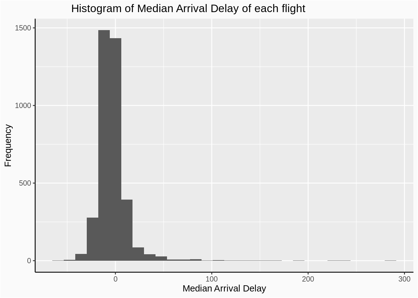
We discover that most flights’ median arrival delay is around 10,while only a very few number of flights have median arrival delay around 75 to 90 minutes.And one or two flights even have median delay over 200 miniutes.
Now let’s plot median arrival delay against number of trips for flight:
not_canceled %>% group_by(flight) %>%
  summarize(count = n(), delay = median(arr_delay)) %>%
  ggplot(aes(x = count, y = delay)) +
  geom_point(alpha = 0.1)+
  labs(x='Number of trips',y='median arrival delay',title='Median Arrival Delay V.s Number of trips')+
  plot_theme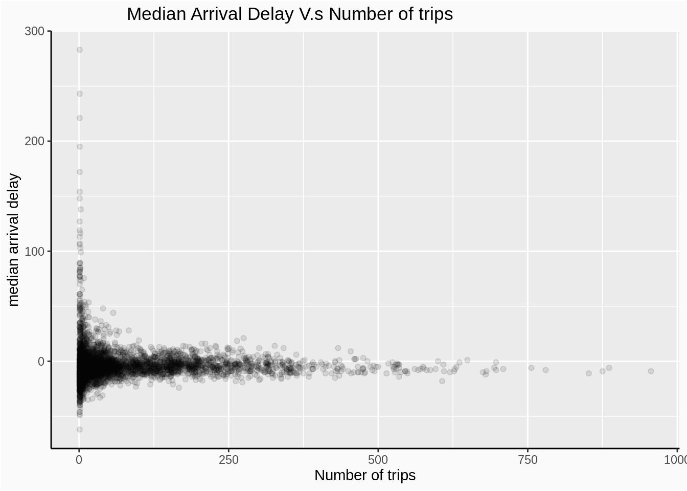
Like the previous plot, we notice that the “outliers” seem to be due to flights with small number of trips. Probably, we should remove them and take a closer look at ones that have more than 25 trips. We also add a regression line with a smoother, hoping to indicate something about relationship between median arrival delay and number of trips of flights.
not_canceled %>% group_by(flight) %>%
  summarize(count = n(), delay = median(arr_delay)) %>%
  filter(count > 25) %>%
  ggplot(aes(x = count, y = delay)) +
  geom_point(alpha = .1) +
  geom_smooth()+
  plot_theme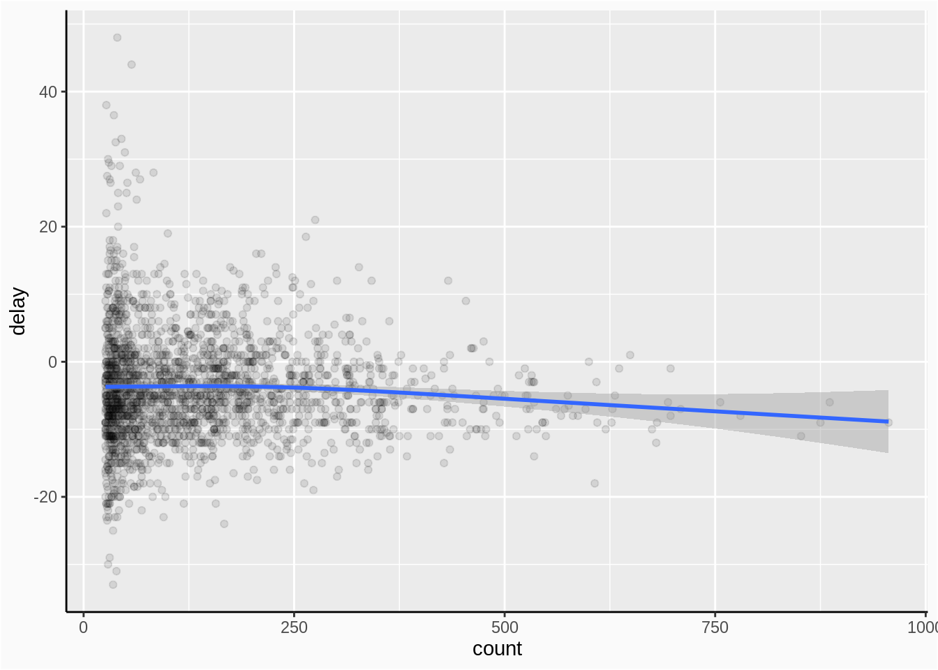
In the plot, we find a very weak negative relationship between number of trips and median arrival delay.
3.5 External Resource
- dplyr: Excellent resource about the overview of dplyr package.
- Linking to URL in markdown and R markdown Cheatsheet: Tools to typeset in markdown.