Chapter 23 Survival analysis examples
Haoxiong Su and Tianchun Huang
23.1 Introduction
Survival analysis is often used to analyze time-to-event data, such as the time that a patient may survive, or the time from HIV infection to development of AIDS. In other words, with survival analysis, we can predict the probability of certain events to happen at certain time, which can be useful in many fields. The objective of this chapter is to introduce some R packages for performing and visualizing survival analysis.
23.2 Basic Concepts
Before introducing R packages, here are some basic concepts and definition about survival analysis.
event: experience of interest, such as death, recovery, and other occurrence.
time \(t\): the time since the beginning of the observation.
censoring: the subject has not experienced the event of interest by the end of data collection, including loss to follow-up, withdrawal from study, or no observation by end.
survival function \(S(t)\): the probability of still being alive at time \(t\); this function is also what we want to estimate in many of the cases.
Kaplan-Meier estimator: Kaplan-Meier survival estimator is an estimate of the survival function derived by Kaplan-Meier method. It is calculated as: \[\hat{S(t_i)} = \prod_{i:t_i\leq t}(1-\frac{d_i}{n_i}),\] where
- \(d_i\): the number of events at \(t_i\)
- \(n_i\): the number of subjects being alive just before \(t_i\)
The R packages we introduce here actually use this method to estimate and plot survival curves.
23.3 Examples
23.3.1 Preparation
23.3.1.1 Load example data
We will use \(cancer\) dataset in \(survival\) package to demonstrate the survival analysis in R:
##   inst time status age sex ph.ecog ph.karno pat.karno meal.cal wt.loss
## 2    3  455      2  68   1       0       90        90     1225      15
## 4    5  210      2  57   1       1       90        60     1150      11
## 6   12 1022      1  74   1       1       50        80      513       0
## 7    7  310      2  68   2       2       70        60      384      10
## 8   11  361      2  71   2       2       60        80      538       1
## 9 1 218 2 53 1 1 70 80 825 16- inst: institution code
- time: survival time
- status: censoring status (1=censored, 2=dead)
- age: age in years
- sex: 1=male, 2=female
- ph.ecog: ECOG performance score (0=good, 5=dead)
- ph.karno: Karnofsky performance score rated by physician (0=bad, 100=good)
- pat.karno: Karnofsky performance score rate by patient
- meal.cal: calories consumed
- wt.loss: weight loss in 6 months
23.3.1.2 Transform the categorical variables
data <- within(data, {
  sex <- factor(sex, labels = c("Male", "Female"))
  ph.ecog <- factor(ph.ecog, labels = c("asymptomatic", "symptomatic", "in bed<50%", "in bed>50%"))
})

head(data)
## inst time status age sex ph.ecog ph.karno pat.karno meal.cal wt.loss
## 2 3 455 2 68 Male asymptomatic 90 90 1225 15
## 4 5 210 2 57 Male symptomatic 90 60 1150 11
## 6 12 1022 1 74 Male symptomatic 50 80 513 0
## 7 7 310 2 68 Female in bed<50% 70 60 384 10
## 8 11 361 2 71 Female in bed<50% 60 80 538 1
## 9 1 218 2 53 Male symptomatic 70 80 825 1623.3.2 Overall Survival analysis
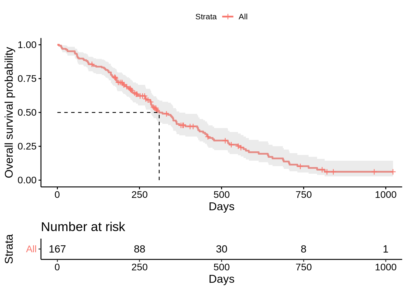
survfit() function fit the Kaplan-Meier curve for the survival data, and ggsurvplot() function visualizes the survival curve.
surv_obj <- survfit(Surv(time, status) ~ 1, data = data)

ggsurvplot(
    fit = surv_obj,
    data = data,
    conf.int = TRUE, # plot the confidence interval of the survival probability
    risk.table = TRUE, # draw the risk table below the graph
    surv.median.line = "hv",# draw the survival median line horizontally & vertically
    xlab = "Days",
    ylab = "Overall survival probability"
    )
23.3.3 Survival analysis between groups
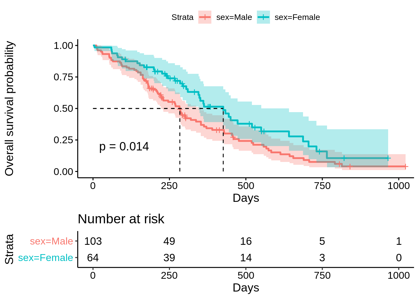
23.3.3.1 Between male and female ECOG performance score
surv_obj <- survfit(Surv(time, status) ~ sex, data = data)
ggsurvplot(
    fit = surv_obj,
    data = data,
    pval = TRUE,  # add the p-value of comparing the differences among groups
    conf.int = TRUE, # plot the confidence interval of the survival probability
    risk.table = TRUE, # draw the risk table below the graph
    surv.median.line = "hv",# draw the survival median line horizontally & vertically
    xlab = "Days",
    ylab = "Overall survival probability",
    tables.height = 0.3
    )
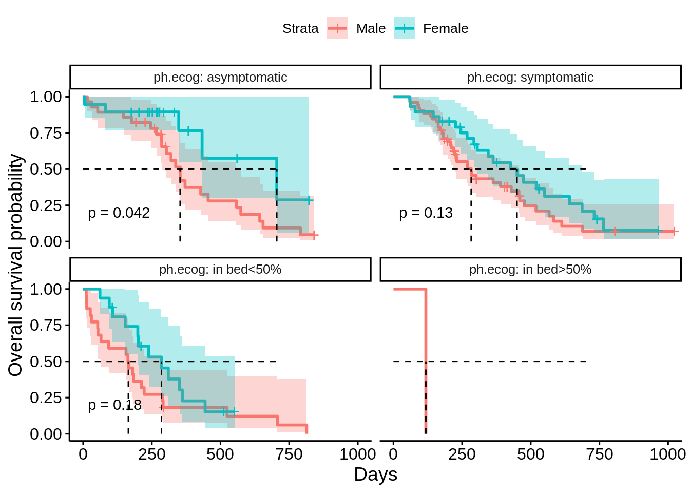
23.3.3.2 Facet by ECOG performance score
surv_obj <- survfit(Surv(time, status) ~ sex, data = data)
ggsurvplot_facet(
    fit = surv_obj,
    data = data,
    facet.by = "ph.ecog",
    pval = TRUE,  # add the p-value of comparing the differences among groups
    conf.int = TRUE, # plot the confidence interval of the survival probability
    surv.median.line = "hv",# draw the survival median line horizontally & vertically
    xlab = "Days",
    ylab = "Overall survival probability",
    tables.height = 0.3
    )
23.3.4 Log-rank test
Log-rank test is a hypothesis test which is often used to compare two survival curves. In the above example, we can use log-rank test to compare the KM curves for male and female. The results below show that p value is 0.001, which means we can reject the null hypothesis and conclude that the survival curves differ in male and female.
## Call:
## survdiff(formula = Surv(time, status) ~ sex, data = lung)
##
##         N Observed Expected (O-E)^2/E (O-E)^2/V
## sex=1 138      112     91.6      4.55      10.3
## sex=2  90       53     73.4      5.68      10.3
##
##  Chisq= 10.3  on 1 degrees of freedom, p= 0.001
23.3.5 Cox model
Cox proportional hazards model is a common approach to analyzing the relationship between the survival of an object and several explanatory variables.
In Cox model, the hazard function is defined as: \[\lambda(t|X_i)=\lambda_0(t)*exp(\beta_1X_{i1}+ \dots+ \beta_pX_{ip})= \lambda_0(t)*exp(X_i*\beta)\]
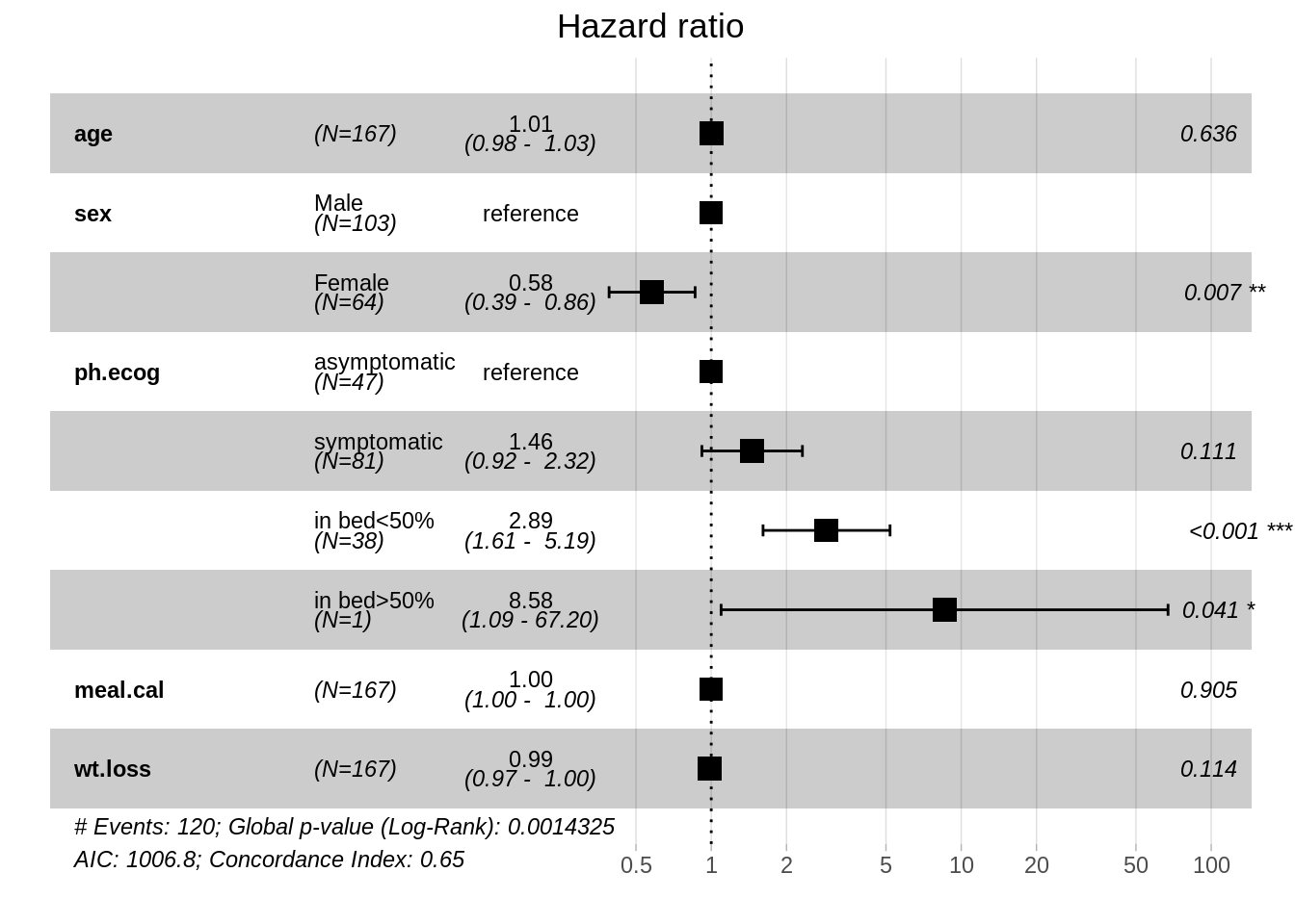
In R, we could use function coxph to create a survival object. After fitting the model, we could use function ggforest to draw the forest plot for Cox model to visualize the effect of each variable.
23.3.5.1 Fit Cox model on only one variable
## Call:
## coxph(formula = Surv(time, status) ~ sex, data = data)
##
##   n= 167, number of events= 120
##
##              coef exp(coef) se(coef)      z Pr(>|z|)
## sexFemale -0.4792    0.6193   0.1966 -2.437   0.0148 *
## ---
## Signif. codes:  0 '***' 0.001 '**' 0.01 '*' 0.05 '.' 0.1 ' ' 1
##
##           exp(coef) exp(-coef) lower .95 upper .95
## sexFemale    0.6193      1.615    0.4212    0.9104
##
## Concordance= 0.567  (se = 0.025 )
## Likelihood ratio test= 6.25  on 1 df,   p=0.01
## Wald test            = 5.94  on 1 df,   p=0.01
## Score (logrank) test = 6.05  on 1 df,   p=0.01