65 Benford Case Study

Abhiram Gaddam, Devan Samant

library(benford.analysis)  #install.packages("benford.analysis")
library(dplyr)
library(plotly)
library(tidyverse)

65.1 Contents

In this tutorial, we will introduce a numeric property called Benford’s Law and illustrate its applications in fraud detection. We will be using the benford_analysis package in R along with an example case study.

Sections:

Introduction
Benford.Analysis Package
Randomized Data Case Study
Conclusion
Sources

65.2 Introduction

There is a niche area of the consulting industry called forensic analytics in which analysts try to identify risks and quantify wrongdoing using an array of statistical and data techniques. For example, imagine a whistleblower notifies a company’s general counsel that there has been some collusion between sales and finance representatives to artificially create invoices. The company may hire forensic analysts to extract and determine what is happening. There are many quantitative and qualitative methods to perform before concluding anything and they will need to be specific to the context of the project. One such heuristic is Benford’s Law.

65.2.1 What is Benford’s Law?

Benford’s law (also known as the first digit law) states that the leading digits in many data sets are probably going to be small. For example, most numbers in a set (about 30%) will have a leading digit of 1, when one might expect the probability to be 11.1% (one out of nine digits). After one, the second most common leading digit is 2 at about 17.5%. And so forth for 3 and onward. To put it simply, Benford’s law is a probability distribution for the likelihood of the first digit in a set of numbers (Frunza, 2015). This pattern is not an intuitive phenomenon but holds true for many naturally occurring datasets (ex. height of mountains around the world) as well as man-made ones such as a company’s general ledger.

The formula for Benford’s Law is: \(P(d) = \frac{ln(1 + \frac{1}{d})}{ln10}\) where \(d\) is the leading digit (a number from 1 to 9)

Below is a distribution that shows the expected occurrence of leading digits according to Benford’s Law.

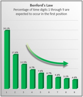
Benfords Law Distribution.

However, there are a few caveats regarding the application of Benford’s Law:

Benford’s Law works better with larger sets of data. While the law has been shown to hold true for data sets containing as few as 50 to 100 numbers, most experts believe data sets of 500 or more numbers are better suited for this type of analysis. (https://tinyurl.com/2p97fsvn)
To conform with the law, the data set you use must contain data in which each number 1 through 9 has an equal chance of occurring as the leading digit. Otherwise, Benford’s Law doesn’t apply. For example, consider a listing of the heights of current NBA players. Since NBA players range in height from 5 feet 10 inches to 7 feet 3 inches, there are no player heights that begin with a 1, 2, 3, 4, 8, or 9; Clearly those digits have no chance of being the first digit in such a listing, making Benford’s Law inapplicable.

While Benford’s Law is not applicable to all datasets, it is generally applicable to large sets of naturally occurring numbers with some connection like:

Companies’ stock market values.
Data found in texts.
Demographic data, including state and city populations.
Income tax data.
Mathematical tables, like logarithms.
River drainage rates.
Scientific data. Benford, F (1938)

65.2.2 Applications in Fraud Detection

One primary and practical use for Benford’s Law is fraud and error detection. It is expected that a large set of numbers will follow the law, so accountants, auditors, economists and tax professionals have a benchmark for what the normal levels of any particular number in a set are. Below are some famously documented examples of Benford’s Law being applied towards fraud detection (Frunza, 2015):

In the 1990s, an accountant named Mark Nigrini found that Benford’s law can be an effective red-flag test for fabricated tax returns. Authentic tax data usually follows Benford’s law, whereas made-up returns do not.
The law was used in 2001 to study economic data from Greece, with the implication that the country may have manipulated numbers to join the European Union.
Ponzi schemes can be detected using the law. Unrealistic returns, such as those purported by the Maddoff scam, fall far from the expected Benford probability distribution .

65.3 Benford Package in R

The Benford Analysis (benford.analysis) package provides tools that make it easier to validate data using Benford’s Law. The main purpose of the package is to identify suspicious data that may need further verification.

Documentation on the package can be found here: https://cran.r-project.org/web/packages/benford.analysis/benford.analysis.pdf

You can install the package from CRAN by running the following (uncommented):

#install.packages("benford.analysis")

The package comes with 6 real datasets from Mark Nigrini’s book Benford’s Law: Applications for Forensic Accounting, Auditing, and Fraud Detection.

65.3.1 Example Usage of benford.analysis

In this section we will give an example using 189,470 records from the corporate payments dataset which is provided with the package.

Load the package and data

data(corporate.payment) 

df <- corporate.payment
head(df)

##   VendorNum       Date  InvNum Amount
## 1      2001 2010-01-02 0496J10  36.08
## 2      2001 2010-01-02 1726J10  77.80
## 3      2001 2010-01-02 2104J10  34.97
## 4      2001 2010-01-02 2445J10  59.00
## 5      2001 2010-01-02 3281J10  59.56
## 6      2001 2010-01-02 3822J10  50.38

To validate the data against Benford’s law you simply use the function “benford” on the appropriate column:

bfd <- benford(df$Amount)
bfd

## 
## Benford object:
##  
## Data: df$Amount 
## Number of observations used = 185083 
## Number of obs. for second order = 65504 
## First digits analysed = 2
## 
## Mantissa: 
## 
##    Statistic  Value
##         Mean  0.496
##          Var  0.092
##  Ex.Kurtosis -1.257
##     Skewness -0.002
## 
## 
## The 5 largest deviations: 
## 
##   digits absolute.diff
## 1     50       5938.25
## 2     11       3331.98
## 3     10       2811.92
## 4     14       1043.68
## 5     98        889.95
## 
## Stats:
## 
##  Pearson's Chi-squared test
## 
## data:  df$Amount
## X-squared = 32094, df = 89, p-value < 2.2e-16
## 
## 
##  Mantissa Arc Test
## 
## data:  df$Amount
## L2 = 0.0039958, df = 2, p-value < 2.2e-16
## 
## Mean Absolute Deviation (MAD): 0.002336614
## MAD Conformity - Nigrini (2012): Nonconformity
## Distortion Factor: -1.065467
## 
## Remember: Real data will never conform perfectly to Benford's Law. You should not focus on p-values!

This creates an object of class “Benford” with the results for the analysis using the first two significant digits by default.

Lets plot the bfd and observe the trends. Note that we running this analysis using the default parameters, i.e., no.of.digits = 2. This parameter can be modified if we only want to analyze the first digit .

plot(bfd)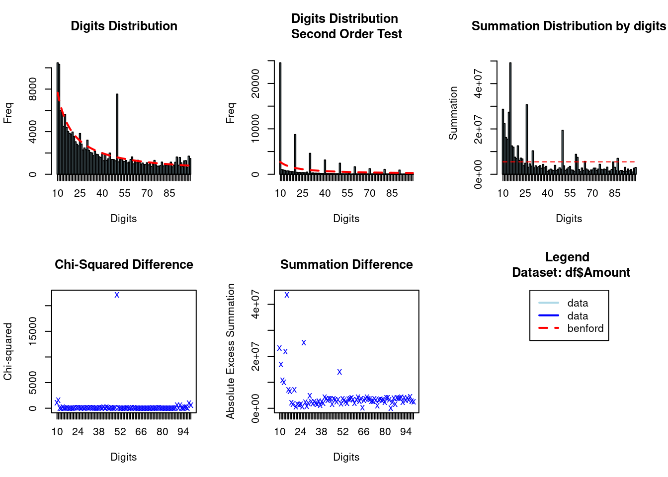

The original data is in blue and the expected frequency according to Benford’s law is in red. In this example, the first plot shows that the data do have a tendency to follow Benford’s law. There is also a clear outlier at 50.

The package also provides some helper functions to further investigate the data. For example, you can easily extract the observations with the largest discrepancies by using the “getSuspects” function.

suspects <- getSuspects(bfd, df)
suspects

##        VendorNum       Date       InvNum  Amount
##     1:      2001 2010-01-02      3822J10   50.38
##     2:      2001 2010-01-07     100107-2 1166.29
##     3:      2001 2010-01-08  11210084007 1171.45
##     4:      2001 2010-01-08      1585J10   50.42
##     5:      2001 2010-01-08      4733J10  113.34
##    ---                                          
## 17852:     52867 2010-07-01 270358343233   11.58
## 17853:     52870 2010-02-01 270682253025   11.20
## 17854:     52904 2010-06-01 271866383919   50.15
## 17855:     52911 2010-02-01 270957401515   11.20
## 17856:     52934 2010-02-01 271745237617   11.88

65.4 Randomized Case Study

In the prior section we saw that when data is manipulated with static values, clearly the first digit rule is broken. But what about when data is randomly manipulated?

Let us try an experiment to see if we can use Benford’s Law to detect potential data manipulation where a bad actor randomly generated fake sales. For this experiment, our baseline will be also be using random data to highlight a point in the conclusion below. Let us pretend a company has sales data comprised of prices and quantities of items that they have sold. This code chunck sets up a data frame where one row is an recorded sale of a number of items sold at a set price.

price <- sample(1:1e3, size = 1e5, replace=TRUE)
quantity <- sample(1:1e4, size = 1e5, replace=TRUE)
df <- data.frame(price,quantity) %>% 
  mutate(value = price*quantity) %>% 
  mutate(digit = substr(as.character(value), 1, 1))

head(df)

##   price quantity   value digit
## 1   382     2174  830468     8
## 2   754     7813 5891002     5
## 3    26     5486  142636     1
## 4   209     9865 2061785     2
## 5   499     8341 4162159     4
## 6   526     4060 2135560     2

Now let us set up and see if this dataset exhibits the expected pattern for the first digit.

df_group <- df %>% group_by(digit) %>% summarise(count = n()) %>%
    mutate(count_percent = count/sum(count))

base_benford = data.frame(c(1,2,3,4,5,6,7,8,9), c(.31,.176,.125,.097,.079,.067,.058,.051,.046))
colnames(base_benford) <- c('digit','percent')

ggplot(data=df_group, aes(x=digit, y=count_percent, fill="blue")) +
  geom_bar(stat="identity", fill='lightblue') + 
  geom_point(aes(x=base_benford$digit, y=base_benford$percent)) +
  scale_y_continuous(labels = scales::percent) +
  labs(title = "First Digit of Randomized Sales",
              subtitle = "Original Data (bar) vs Expected Benford (point)",
              #caption = "TBD",
              x = "First Digit", y = "% Occurance",
              #tag = "A"
              ) +  theme(legend.position="none")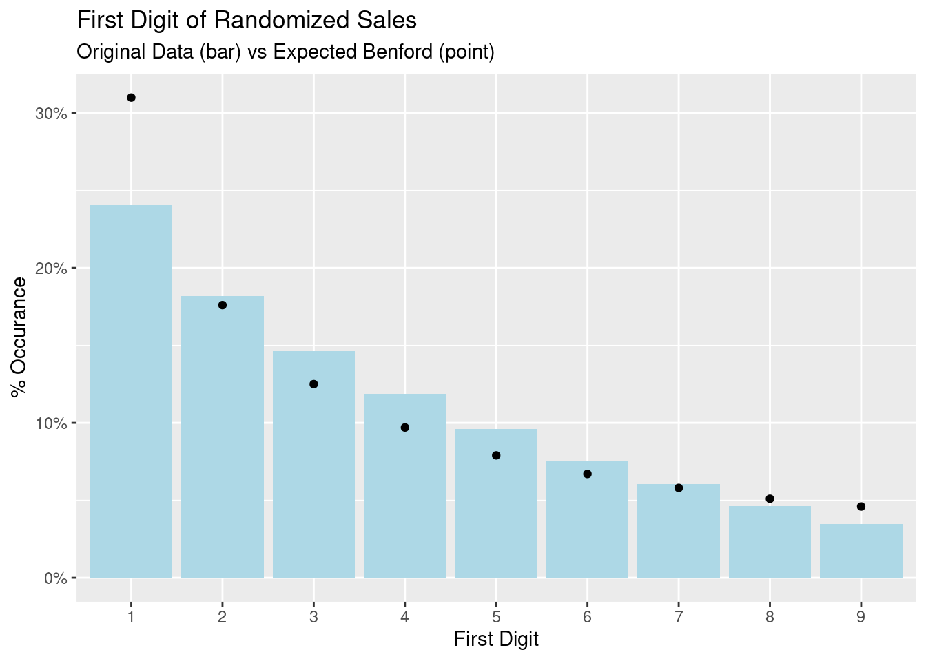

The [value] of the sales exhibits some commonality with Benford’s Law but it is not exact as we see the first digit is not quite 30%. However there is still that decreasing probability of the leading digit. We will address some limitation in the next section. For now, let us try manipulating the data to see if any patterns change.

65.4.1 Manipulated Data

In this next piece of code, we can pretend someone has entered in additional sales “randomly” by adding lots of relatively smaller sales under 100k.

value2 <- sample(1:1e6, size = 4e5, replace=TRUE)
df_extra_sales <- data.frame(0,0,value2)
colnames(df_extra_sales) <- c('price','quantity','value')
df2 <- data.frame(price,quantity) %>% 
  mutate(value = price*(quantity)) %>% 
  rbind(df_extra_sales)  %>% 
  mutate(digit = substr(as.character(value), 1, 1))

df_group2 <- df2 %>% group_by(digit) %>% summarise(count = n()) %>%
    mutate(count_percent = count/sum(count))

df_group_combined <- data.frame(df_group$digit,df_group$count_percent,df_group2$count_percent) 
colnames(df_group_combined) <- c('digit','Original','Manipulated')
df_group_combined <- df_group_combined %>% pivot_longer(cols=c('Original','Manipulated'))
colnames(df_group_combined) <- c('digit','Dataset','count_percent')

ggplot(data=df_group_combined, aes(x=digit, y=count_percent, fill=fct_rev(as.factor(Dataset)) )) +
  geom_bar(stat="identity", position='dodge') +
  scale_y_continuous(labels = scales::percent) +
  labs(title = "First Digit of Manipulated Sales",
              subtitle = "Original Data vs Manipulated Data",
              x = "First Digit", y = "% Occurance",
              fill="Dataset"
              ) +  theme(legend.position="bottom")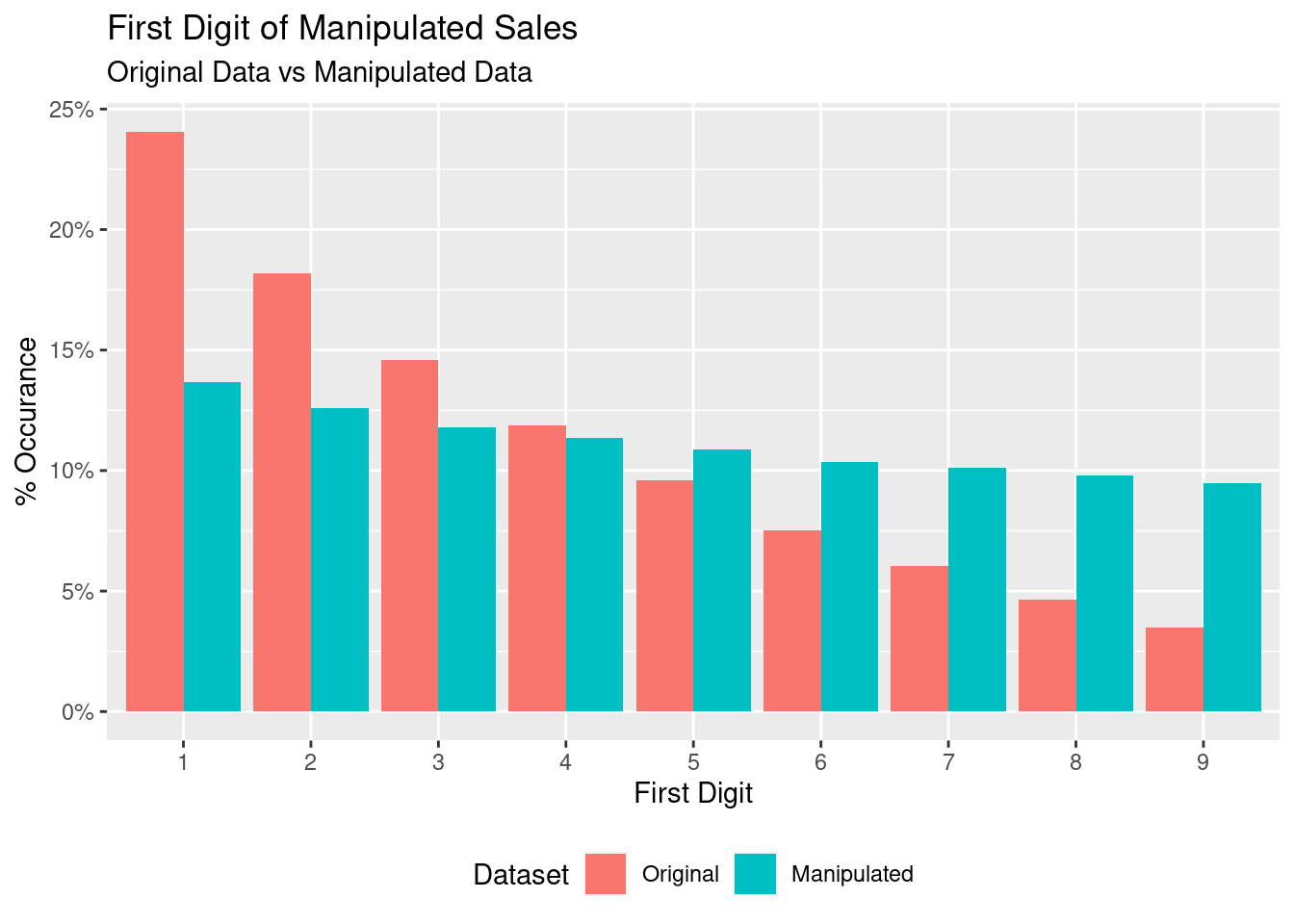

From here we can see that adding sales randomly does change the distribution (when enough of them are added). But can we quantify this change? Let us use the benford package to cacluate some statistics. The following

bfd_1 <- benford(df$value)
#bfd_1

bfd_2 <- benford(df2$value)
#bfd_2

Printing the benford object creates verbose output so we have copied the main statistics below between the two dataframes:

bfd_1 (df - original) Statistic Value Mean 0.526 Var 0.073 Ex.Kurtosis -1.048 Skewness -0.145

bfd_1 (df2 - manipulated) Statistic Value Mean 0.65 Var 0.07 Ex.Kurtosis -0.59 Skewness -0.66

If the data follows Benford’s Law, the expected statistics should be close to: Statistic Value Mean 0.5 Var 0.083 Ex.Kurtosis -1.2 Skewness 0

From a glance, it is evident that the statistics corresponding to the original df are much closer to the expected statistics than those from df2. In particular, the Ex.Kurtosis and Skewness differ significantly in df2 from the expected values. These are all indicators that the set of values deviate from the expected distribution corresponding to Benford’s Law.

65.4.2 Findings

So what does this show us? If both sets were randomly generated, why would one not conform to Benford’s Law? One reason is that data that is the product of many random variables tends to exhibit a log-normal distribution which fits well with the first digit rule. However, by adding values in a static way, we change the data to be more uniform and distort the decaying curve.

Now it is important to understand that 1) this case is an extreme example to highlight a point, and 2) that Benford’s Law and its statistics do not prove anything - they only provide some guidance on areas that may look strange. In reality, forensic testing would be done on specific segments or accounts, people would be interviewed, systems and logs analyzed, etc. Similarly, even when Benford’s Law holds true, it does not mean there is no fraud; a bad actor that understands fraud detection methods will likely hide better.

65.5 Conclusion

An important thing to note is that Benford’s law does not have a strict mathematical proof, and is simply a heuristic. It is a broad guideline which helps with the investigation of large data sets to see if they conform with the observed trends. A feature of a dataset that conforms with Benford’s Law is not proof of validity or vice versa. For this reason, a Benford analysis is usually conducted as a primary investigatory exercise, following which a more thorough investigation as described in the previous section is conducted.

65.6 Sources

Benford, F. “The Law of Anomalous Numbers,” Proceedings of the American Philosophical Society, 78, 551–572. 1938.

Frunza, M. (2015). Solving Modern Crime in Financial Markets: Analytics and Case Studies. Academic Press.

https://cran.r-project.org/web/packages/benford.analysis/benford.analysis.pdf

https://www.statisticshowto.com/benfords-law/

https://tinyurl.com/2p97fsvn

63 How I got into Amazon as a full time data analyst

67 Equity in AI