25 Tutorial for vector fields in r

Sebastian Steiner & Elliot Frank

25.1 Getting Started with Vector Fields

Vector field graphs have a number of important applications throughout science, engineering, and math. In this tutorial, we’ll explain the basic components of vector field graphs, and how to build them in R.

From our research, the documentation available could use improvement, and thus our goal is provide an accessible explanation of how to build vector graphs in R. To keep things clear, we’ll build an example data set as we go, explaining all of the required data components of vector field graphs. Hopefully, after reading this tutorial, you’ll be able to easily put together vector graphs using other data sets.

In our example data set, each observation represents one arrow, or vector, to be plotted on the graph. As vectors communicate movement, each arrow will have a starting point and an end point. Before we dive in, we’ve listed below the four data columns required for building a vector graph, each of which we will build in our example data set.

x_axis: horizontal value of the starting point for a given vector
y_axis: vertical value of the starting point for a given vector
x_pull: strength of force pulling vector in horizontal direction
y_pull: strength of force pulling vector in vertical direction

First, we will require two data columns serving as x and y coordinates for placement of the arrow on the graph. These initial coordinates, which we will call x_axis and y_axis, will place the base of each arrow on the vector graph. Stated otherwise, together the x_axis and y_axis columns provide the starting point for each arrow on the graph.

In the code below, we start building our example data set by placing the base of each vector on all positive integer values of a 10 X 10 grid, by assigning values to the x_axis and y_axis columns.

# Creating a blank data frame with four required columns
data_frame = data.frame(x_axis = numeric(), y_axis = numeric())

# Generating evenly distributed values for x y coordinates
for(i in 1:10) {
  for(j in 1:10) {
    vec <- c(i, j) 
    data_frame[nrow(data_frame) + 1, ] <- vec
  }
}

# Plotting points for illustrative purposes
ggplot(data_frame, aes(x = x_axis, y = y_axis)) +
    scale_x_continuous(breaks = seq(0,10,1)) + 
    scale_y_continuous(breaks = seq(0,10,1)) +
    geom_segment(aes(xend = x_axis+(0.05), yend = y_axis)) +
    coord_fixed()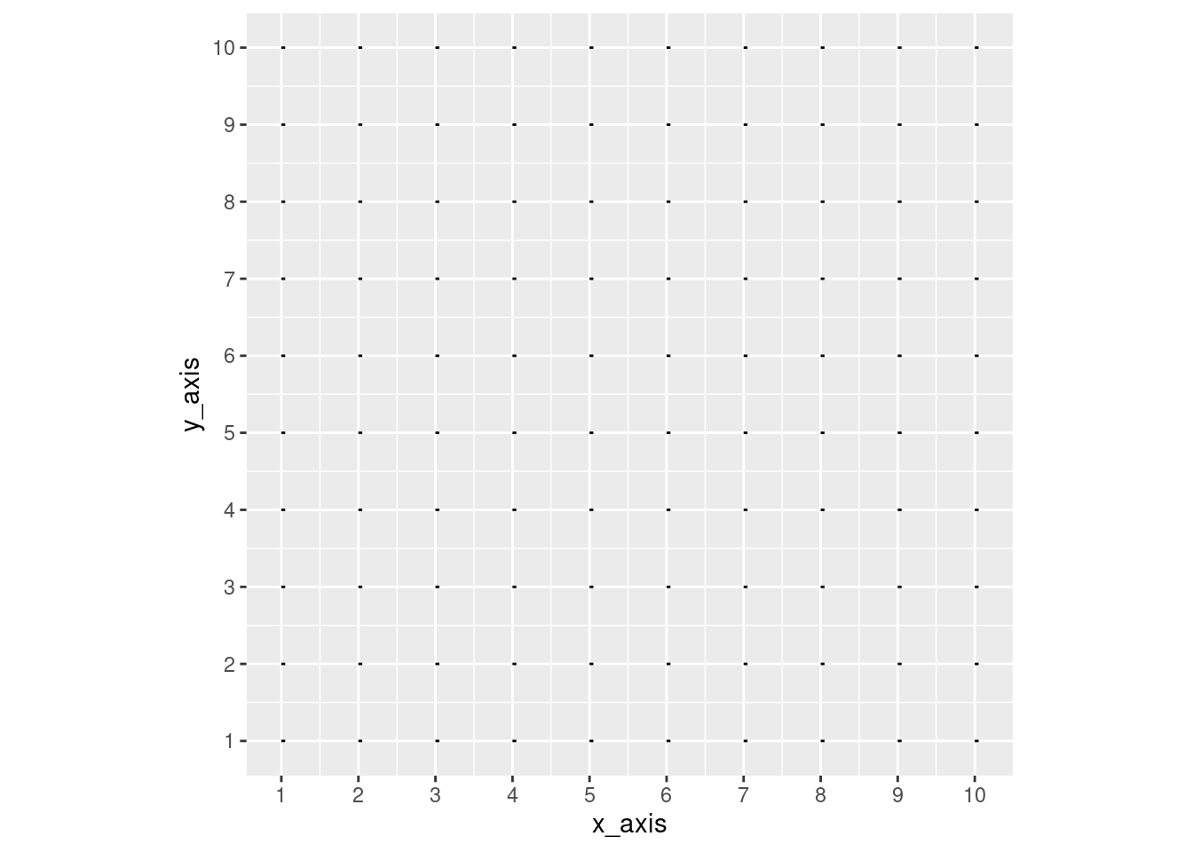

In graphing the plot, we’ve assigned the x_axis and y_axis values as the axis values of the entire chart, again, as the columns place each arrow. The geom_segment function plots the lines, we’ve added an endpoint of 0.05 to the x_axis so that the base of each vector can be seen above.

After plotting the starting points of all vectors, we now need to determine where all of our vectors will end. This will be determined by the x_pull and y_pull columns. It’s important to note that these columns will not provide the end coordinates, but a measure of the directions in which each vector is pulled. The x_pull and y_pull variables will indicate how far from the base the arrow should extend in the given direction.

You’ll notice in the code below, the x_pull and y_pull values are being added to the starting point values (x_axis & y_axis) in the geom_segment function. The variables within ‘aes’, which dictate the end points of a vector, are conveniently named ‘xend’ and ‘yend’. By altering the ‘xend’ and ‘yend’ values, we place the coordinates of a vector’s endpoint.

For example, if I set only the y_pull equal to 0.5, you’ll notice that all of the arrows are being pulled in an upward direction.

data_frame$x_pull <- 0
data_frame$y_pull <- 0.5

# Plotting points for illustrative purposes
ggplot(data_frame, aes(x = x_axis, y = y_axis)) +
    scale_x_continuous(breaks = seq(0,10,1)) + 
    scale_y_continuous(breaks = seq(0,10,1)) +
    geom_segment(aes(xend = x_axis + (x_pull), 
                     yend = y_axis + (y_pull)), 
                 arrow = arrow(length = unit(0.1, "cm")), size = 0.25) +
    coord_fixed()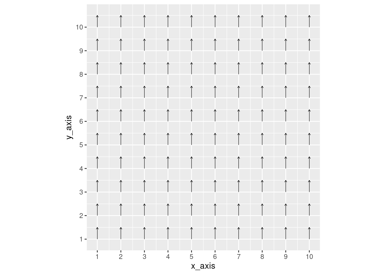

Conversely, if I set only the x_pull equal to 0.5, you’ll notice that all of the arrows are being pulled to the right direction.

data_frame$x_pull <- 0.5
data_frame$y_pull <- 0

# Plotting points for illustrative purposes
ggplot(data_frame, aes(x = x_axis, y = y_axis)) +
    scale_x_continuous(breaks = seq(0,10,1)) + 
    scale_y_continuous(breaks = seq(0,10,1)) +
    geom_segment(aes(xend = x_axis + (x_pull), 
                     yend = y_axis + (y_pull)), 
                 arrow = arrow(length = unit(0.1, "cm")), size = 0.25) +
    coord_fixed()

If we set both x_pull and y_pull equal to 0.5, then the x and y forces are offsetting, and the arrows point in a 45 degree angle.

data_frame$x_pull <- 0.5
data_frame$y_pull <- 0.5

ggplot(data_frame, aes(x = x_axis, y = y_axis)) +
    scale_x_continuous(breaks = seq(0,10,1)) + 
    scale_y_continuous(breaks = seq(0,10,1)) +
    geom_segment(aes(xend = x_axis + (x_pull), 
                     yend = y_axis + (y_pull)), 
                     arrow = arrow(length = unit(0.1, "cm")), size = 0.25) +
    coord_fixed()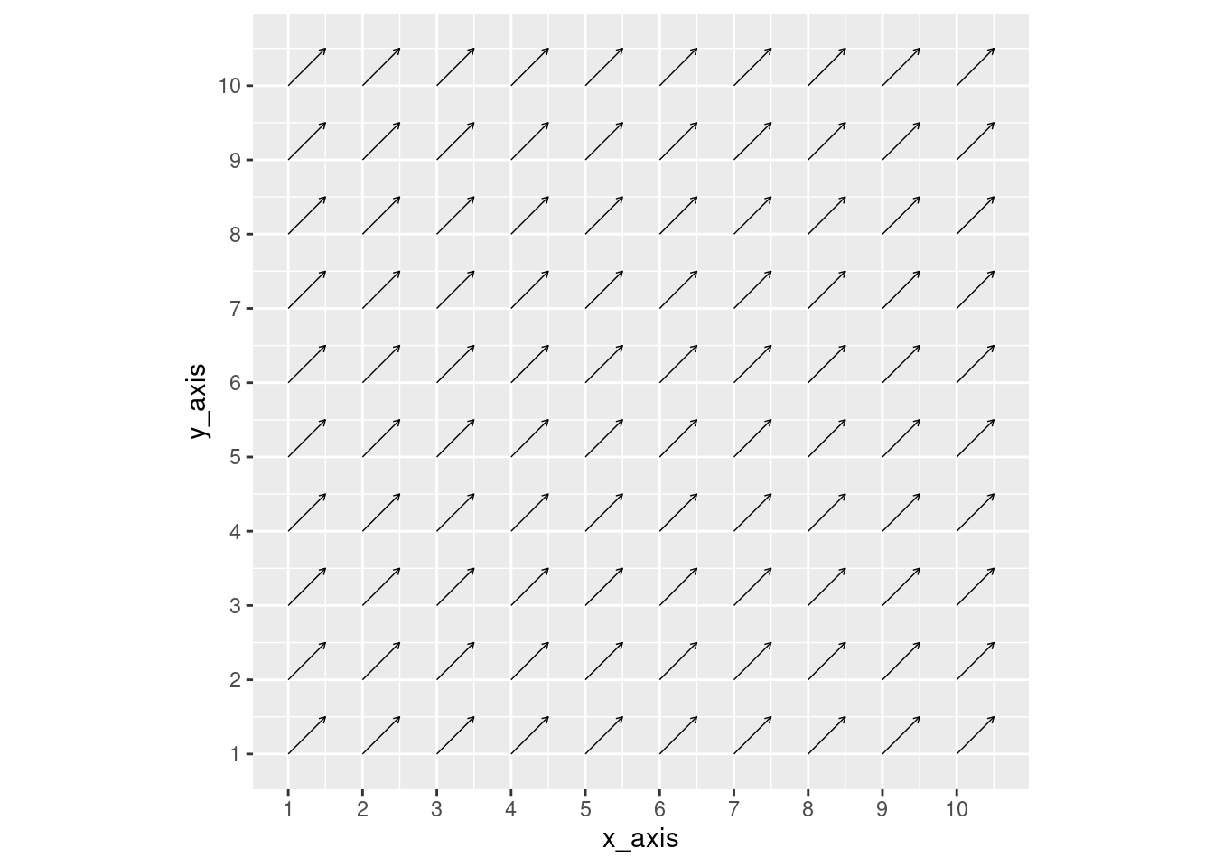

To provide another example, we’ve input random numbers into x_pull and y_pull values, to show that the format is completely flexible and doesn’t require consistent value changes to the x_pull and y_pull variables.

data_frame$x_pull <- runif(nrow(data_frame), min=-0.5, max=0.5)
data_frame$y_pull <- runif(nrow(data_frame), min=-0.5, max=0.5)

ggplot(data_frame, aes(x = x_axis, y = y_axis)) +
    scale_x_continuous(breaks = seq(0,10,1)) + 
    scale_y_continuous(breaks = seq(0,10,1)) +
    geom_segment(aes(xend = x_axis + (x_pull), 
                     yend = y_axis + (y_pull)), 
                     arrow = arrow(length = unit(0.1, "cm")), size = 0.25) +
    coord_fixed()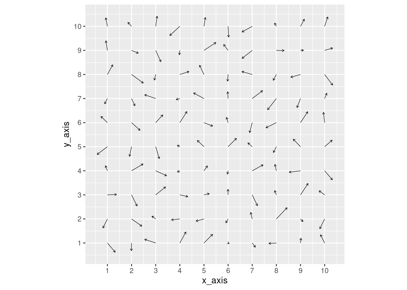

25.2 Tips and Tricks to Plotting Vector Fields

Now that we’ve covered the basics, we’ll provide guidance on how to make high-quality vector field graphs.

25.2.1 Understanding arrow options

When plotting arrows in geom_segment, we can control some features of the arrow in the following line:

arrow = arrow(length = unit(0.1, "cm")), size = 0.25)

length = unit(0.1, “cm”) defines the size of the arrow head
size = 0.25 defines arrow thickness

For example, if we set both to 1, we get the following:

data_frame$x_pull <- 0.5
data_frame$y_pull <- 0.5

ggplot(data_frame, aes(x = x_axis, y = y_axis)) +
    scale_x_continuous(breaks = seq(0,10,1)) + 
    scale_y_continuous(breaks = seq(0,10,1)) +
    geom_segment(aes(xend = x_axis + (x_pull), 
                     yend = y_axis + (y_pull)), 
                     arrow = arrow(length = unit(1, "cm")), size = 1) +
    coord_fixed()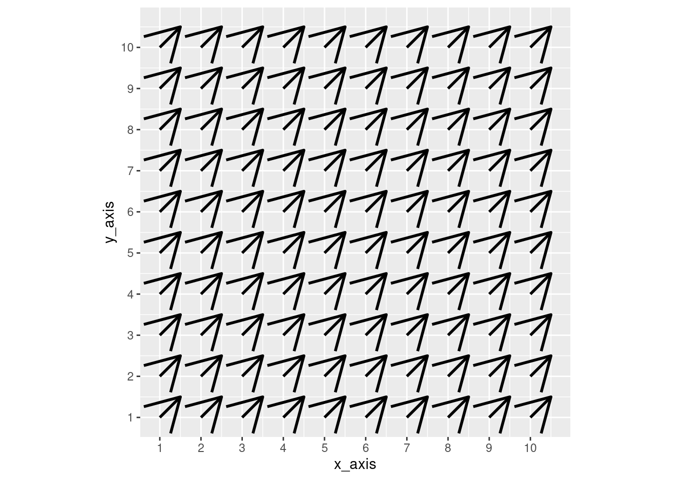

These arrow adjustments produce a low-quality plot, but they do highlight the options one has to represent arrows in vector fields.

25.2.2 Axis Scaling

Vector fields commonly represent flows in space. Therefore, moving 1 unit in the x-direction has the same distance as moving 1 unit in the y-direction. If this 1:1 ratio is not preserved, the vector field becomes distorted and difficult to interpret. Therefore, the axis in ggplot must be fixed using the following code:

coord_fixed()

Below is an illustration of this discussion - note in both cases, all vectors have the form (0.5,0.5). While the distortion appears to be small, it is easily avoidable and preserves an accurate relationship between the x and y axes.

#Creating homogeneous vector field (1,1)
data_frame$x_pull <- 0.5
data_frame$y_pull <- 0.5

#No coord_fixed
ggplot(data_frame, aes(x = x_axis, y = y_axis)) +
  scale_x_continuous(breaks = seq(0,10,1)) + 
  scale_y_continuous(breaks = seq(0,10,1)) +
  geom_segment(aes(xend = x_axis + (x_pull), 
                  yend = y_axis + (y_pull)), 
                  arrow = arrow(length = unit(0.1, "cm")), size = 0.25)  +
  ggtitle("Distorted plot without coord_fixed()")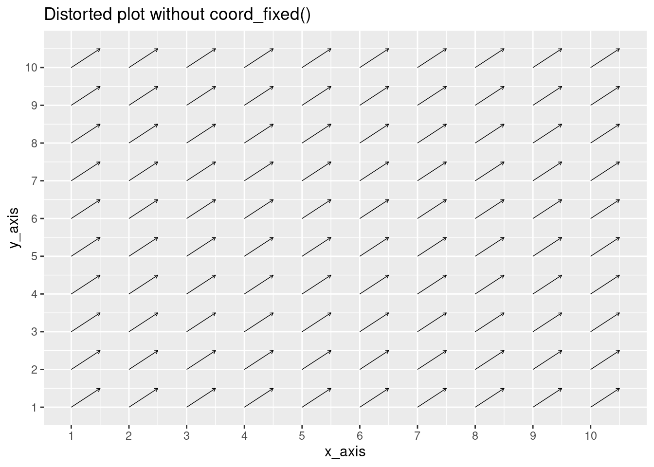

#Coord_fixed
ggplot(data_frame, aes(x = x_axis, y = y_axis)) +
        scale_x_continuous(breaks = seq(0,10,1)) + 
        scale_y_continuous(breaks = seq(0,10,1)) +
        geom_segment(aes(xend = x_axis + (x_pull), 
                        yend = y_axis + (y_pull)), 
                        arrow = arrow(length = unit(0.1, "cm")), size = 0.25) +
        coord_fixed() +
        ggtitle("High-quality plot with coord_fixed()")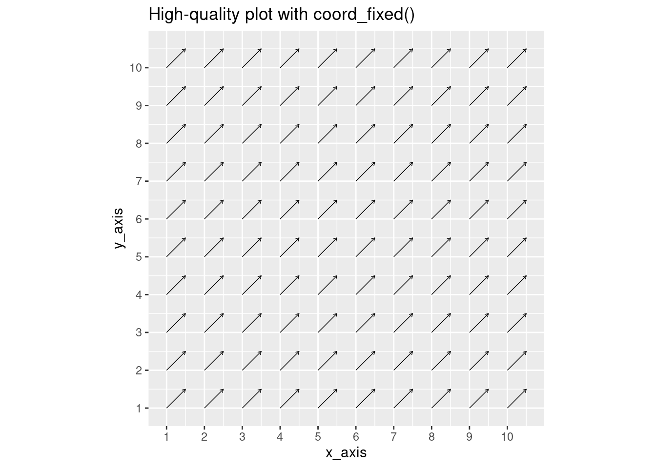

25.2.3 Arrow Length

It is important to consider the length of arrows when plotting vector fields, as input data may cause arrows to overlap, making the plot difficult to interpret (see example below).

data_frame$x_pull <- 5
data_frame$y_pull <- 1

# Plotting points for illustrative purposes
ggplot(data_frame, aes(x = x_axis, y = y_axis)) +
    scale_x_continuous(breaks = seq(0,10,1)) + 
    scale_y_continuous(breaks = seq(0,10,1)) +
    geom_segment(aes(xend = x_axis + (x_pull), 
                     yend = y_axis + (y_pull)), 
                 arrow = arrow(length = unit(0.1, "cm")), size = 0.25) +
    coord_fixed()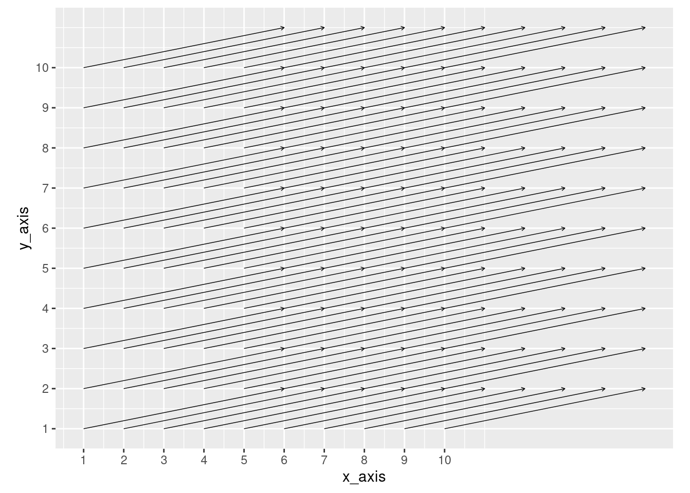

As you can see, even with a simple plot that has all vectors pointing in the same direction, overlapping arrows makes it impossible to see the origin point of arrows in the middle. Therefore, we recommend scaling down the x_pull and y_pull vectors, as shown below (note it is good practice to scale the x_pull and y_pull by the same amount).

# Assume this is the raw x_pull & y_pull data
data_frame$x_pull <- 5
data_frame$y_pull <- 1

# Scale vector data
data_frame$x_pull <- data_frame$x_pull / 10
data_frame$y_pull <- data_frame$y_pull / 10

# Plotting points for illustrative purposes
ggplot(data_frame, aes(x = x_axis, y = y_axis)) +
    scale_x_continuous(breaks = seq(0,10,1)) + 
    scale_y_continuous(breaks = seq(0,10,1)) +
    geom_segment(aes(xend = x_axis + (x_pull), 
                     yend = y_axis + (y_pull)), 
                 arrow = arrow(length = unit(0.1, "cm")), size = 0.25) +
    coord_fixed()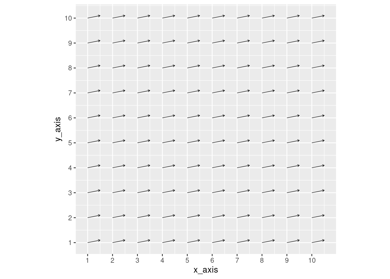

25.2.4 Arrow Color

When scaling down the arrows, the absolute length of the arrows loses meaning, and distorts the relative strength of vectors in the graph. While this qualitative representation is acceptable in most cases of plotting vector fields, it is possible to add color to arrows based on their magnitude - see below. Moreover, above the color bar we can add a title explaining the units that the colors represent (e.g. m/s). For this example, we’ll create a new data set with x_axis and y_axis values ranging from -10 to 10.

vector_frame = data.frame(x_axis = numeric(), y_axis = numeric())

# Generating evenly distributed values for x y coordinates
for(i in -10:10) {
  for(j in -10:10) {
    vec <- c(i, j) 
    vector_frame[nrow(vector_frame) + 1, ] <- vec
  }
}

vector_frame$x_pull <- with(vector_frame, -x_axis/(sqrt((x_axis^2) + (y_axis^2)) + 4))
vector_frame$y_pull <- with(vector_frame, 2*y_axis/(sqrt((x_axis^2) + (y_axis^2)) + 4))
vector_frame$mag    <- sqrt( (vector_frame$x_pull^2) + (vector_frame$y_pull)^2 ) 

ggplot(vector_frame, aes(x = x_axis, y = y_axis, colour=mag) )+
    scale_colour_continuous(name = "*Units") +
    scale_x_continuous(breaks = seq(-10,10,1)) + 
    scale_y_continuous(breaks = seq(-10,10,1)) +
    geom_segment(aes(xend = x_axis + (x_pull), 
                     yend = y_axis + (y_pull)), 
                     arrow = arrow(length = unit(0.1, "cm")), size = 0.25) +
    geom_vline(xintercept=0, size=0.15) + geom_hline(yintercept=0, size=0.15) +
    coord_fixed()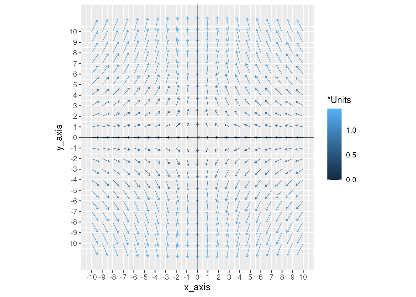

In the following plot, we have changed the arrow color to be based on the x_pull value, rather than magnitude. This could be useful if the flow in one direction is more important than the other.

vector_frame = data.frame(x_axis = numeric(), y_axis = numeric())

# Generating evenly distributed values for x y coordinates
for(i in -10:10) {
  for(j in -10:10) {
    vec <- c(i, j) 
    vector_frame[nrow(vector_frame) + 1, ] <- vec
  }
}

vector_frame$x_pull <- with(vector_frame, -x_axis/(sqrt((x_axis^2) + (y_axis^2)) + 4))
vector_frame$y_pull <- with(vector_frame, 2*y_axis/(sqrt((x_axis^2) + (y_axis^2)) + 4))

ggplot(vector_frame, aes(x = x_axis, y = y_axis, colour=x_pull) )+
    scale_colour_continuous(low = "dodgerblue", high = "darkred") +
    scale_x_continuous(breaks = seq(-10,10,1)) + 
    scale_y_continuous(breaks = seq(-10,10,1)) +
    geom_segment(aes(xend = x_axis + (x_pull), 
                     yend = y_axis + (y_pull)), 
                     arrow = arrow(length = unit(0.1, "cm")), size = 0.25) +
    geom_vline(xintercept=0, size=0.15) + geom_hline(yintercept=0, size=0.15) +
    coord_fixed()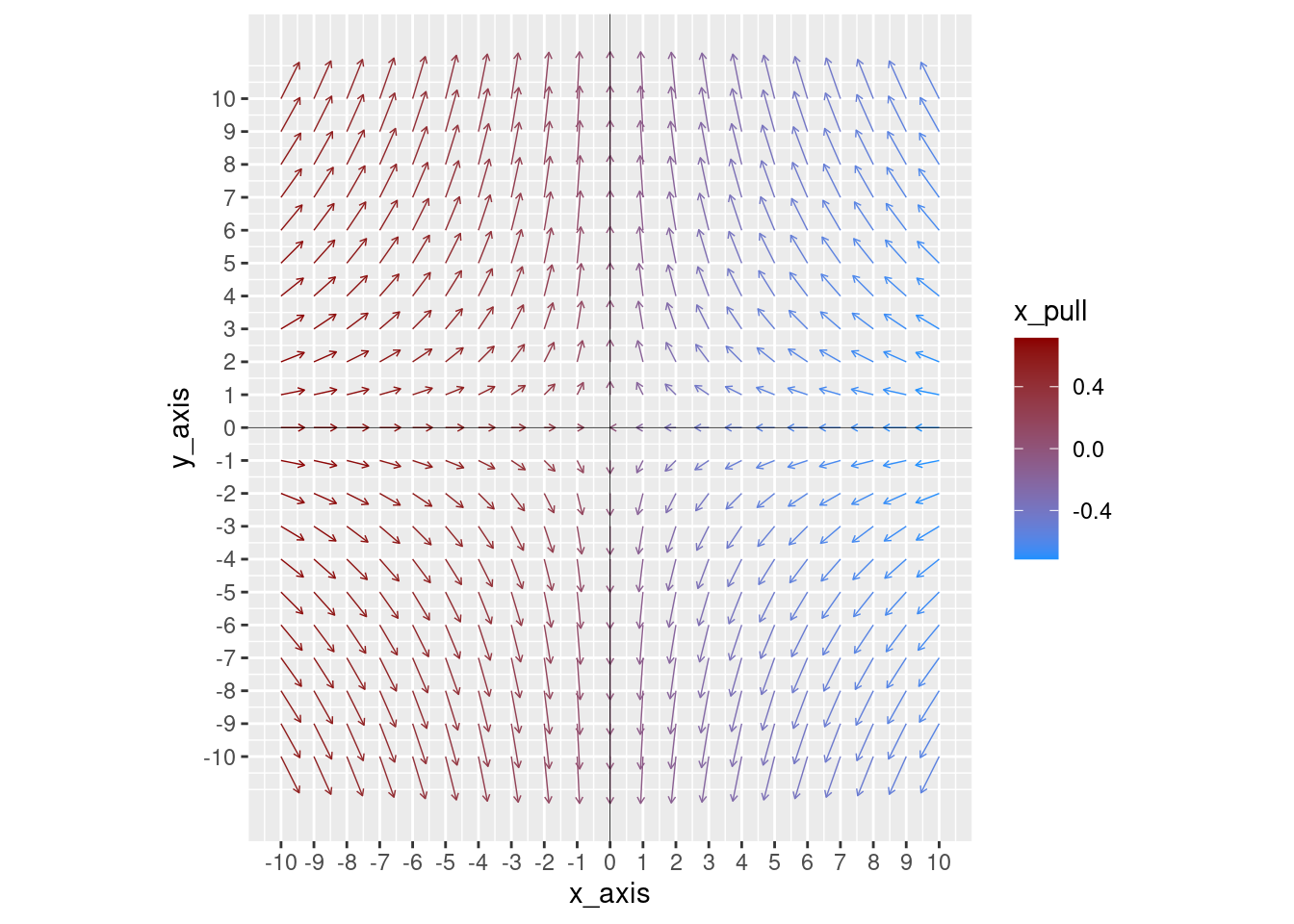

25.3 Spacing

Vector fields often describe flows in continuous space, which means there could be an infinite number of vectors in the plot. To overcome this, we usually sample uniformly spaced points in the field and plot their vectors. Choosing the point spacing is important because if we down-sample too much, we lose information. On the other hand if, don’t down-sample enough, the vector field becomes cluttered.

vector_frame1 = data.frame(x_axis = numeric(), y_axis = numeric())

# Generating a dense vector field
for(i in seq(-10, 10, by=0.4)) {
  for(j in seq(-10, 10, by=0.4)) {
    vec <- c(i, j) 
    vector_frame1[nrow(vector_frame1) + 1, ] <- vec
  }
}

vector_frame1$x_pull <- with(vector_frame1, -x_axis/(sqrt((x_axis^2) + (y_axis^2)) + 4))
vector_frame1$y_pull <- with(vector_frame1, 2*y_axis/(sqrt((x_axis^2) + (y_axis^2)) + 4))

p1 <- ggplot(vector_frame1, aes(x = x_axis, y = y_axis) )+
        scale_x_continuous(breaks = seq(-10,10,2)) + 
        scale_y_continuous(breaks = seq(-10,10,2)) +
        geom_segment(aes(xend = x_axis + (x_pull), 
                         yend = y_axis + (y_pull)), 
                         arrow = arrow(length = unit(0.1, "cm")), size = 0.25) +
        geom_vline(xintercept=0, size=0.15) + geom_hline(yintercept=0, size=0.15) +
        ggtitle("Not enough spacing") +
        theme(text=element_text(size=9)) +
        coord_fixed()

vector_frame2 = data.frame(x_axis = numeric(), y_axis = numeric())

# Generating a sparse vector field
for(i in seq(-10, 10, by=5)) {
  for(j in seq(-10, 10, by=5)) {
    vec <- c(i, j) 
    vector_frame2[nrow(vector_frame2) + 1, ] <- vec
  }
}

vector_frame2$x_pull <- with(vector_frame2, -x_axis/(sqrt((x_axis^2) + (y_axis^2)) + 4))
vector_frame2$y_pull <- with(vector_frame2, 2*y_axis/(sqrt((x_axis^2) + (y_axis^2)) + 4))

p2 <- ggplot(vector_frame2, aes(x = x_axis, y = y_axis) )+
        scale_x_continuous(breaks = seq(-10,10,2)) + 
        scale_y_continuous(breaks = seq(-10,10,2)) +
        geom_segment(aes(xend = x_axis + (x_pull), 
                         yend = y_axis + (y_pull)), 
                         arrow = arrow(length = unit(0.1, "cm")), size = 0.25) +
        geom_vline(xintercept=0, size=0.15) + geom_hline(yintercept=0, size=0.15) +
        ggtitle("Too much spacing") +
        theme(text=element_text(size=9)) +
        coord_fixed()

p1 + p2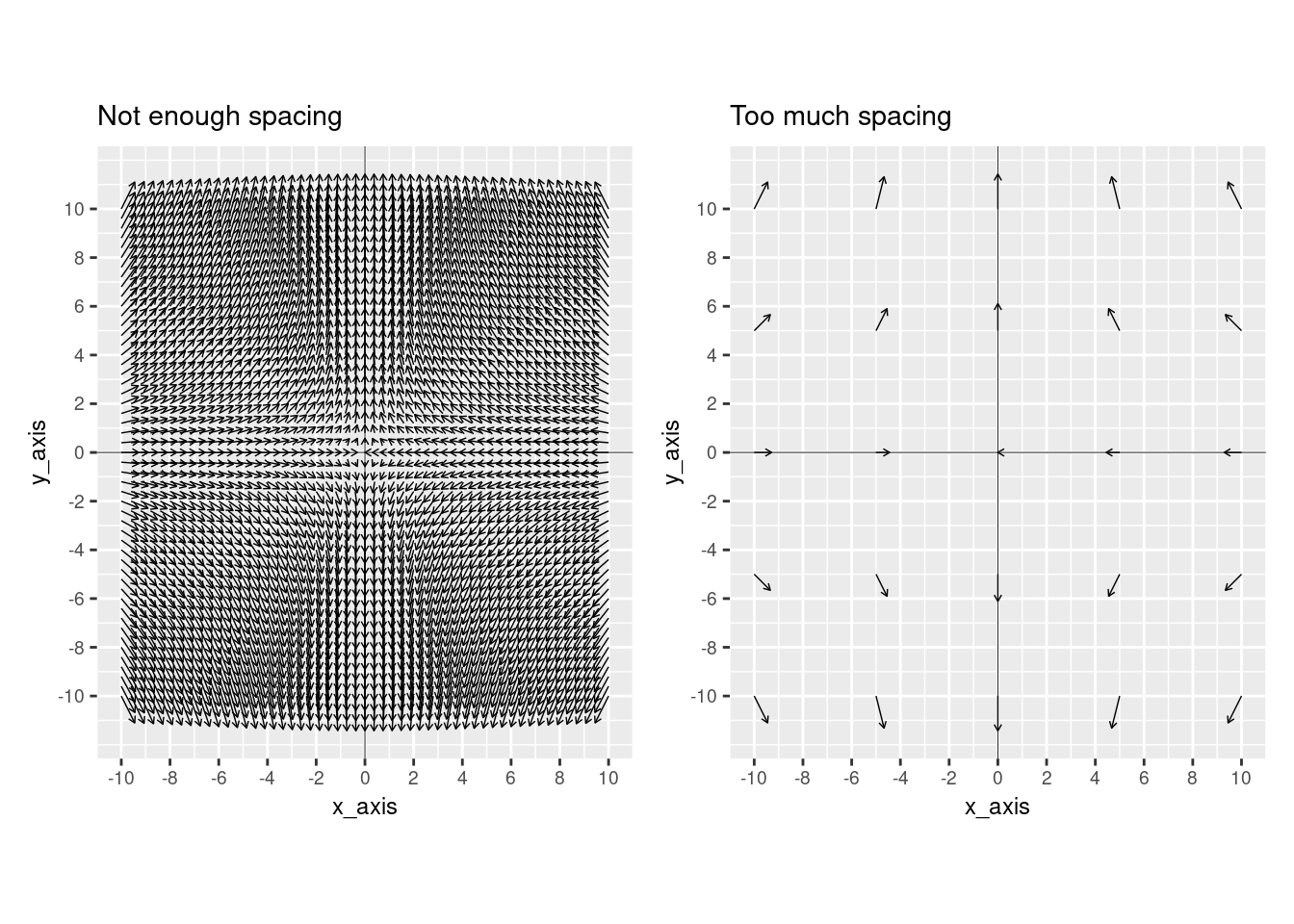

As shown above, at the extremes of spacing, vector fields are difficult to interpret. Hence, there must be an optimal spacing between the two. As illustrated below, this optimal spacing also depends on arrow length because closer spacing requires shorter arrow lengths, while larger spacing allows longer arrow lengths. In other words, there is a trade-off between vector spacing and vector length.

vector_frame1 = data.frame(x_axis = numeric(), y_axis = numeric())

# Vector field with larger spacing and arrows

for(i in seq(-10, 10, by=2)) {
  for(j in seq(-10, 10, by=2)) {
    vec <- c(i, j) 
    vector_frame1[nrow(vector_frame1) + 1, ] <- vec
  }
}

vector_frame1$x_pull <- with(vector_frame1, -2*x_axis/(sqrt((x_axis^2) + (y_axis^2)) + 4))
vector_frame1$y_pull <- with(vector_frame1, 3*y_axis/(sqrt((x_axis^2) + (y_axis^2)) + 4))

p1 <- ggplot(vector_frame1, aes(x = x_axis, y = y_axis) )+
        scale_x_continuous(breaks = seq(-10,10,2)) + 
        scale_y_continuous(breaks = seq(-10,10,2)) +
        geom_segment(aes(xend = x_axis + (x_pull), 
                         yend = y_axis + (y_pull)), 
                         arrow = arrow(length = unit(0.1, "cm")), size = 0.25) +
        geom_vline(xintercept=0, size=0.15) + geom_hline(yintercept=0, size=0.15) +
        ggtitle("Opitmal with more spacing") +
        theme(text=element_text(size=9)) +
        coord_fixed()

vector_frame2 = data.frame(x_axis = numeric(), y_axis = numeric())

# Vector field with smaller spacing and arrows

for(i in seq(-10, 10, by=1)) {
  for(j in seq(-10, 10, by=1)) {
    vec <- c(i, j) 
    vector_frame2[nrow(vector_frame2) + 1, ] <- vec
  }
}

vector_frame2$x_pull <- with(vector_frame2, -x_axis/(sqrt((x_axis^2) + (y_axis^2)) + 4))
vector_frame2$y_pull <- with(vector_frame2, y_axis/(sqrt((x_axis^2) + (y_axis^2)) + 4))

p2 <- ggplot(vector_frame2, aes(x = x_axis, y = y_axis) )+
        scale_x_continuous(breaks = seq(-10,10,2)) + 
        scale_y_continuous(breaks = seq(-10,10,2)) +
        geom_segment(aes(xend = x_axis + (x_pull), 
                         yend = y_axis + (y_pull)), 
                         arrow = arrow(length = unit(0.1, "cm")), size = 0.25) +
        geom_vline(xintercept=0, size=0.15) + geom_hline(yintercept=0, size=0.15) +
        ggtitle("Optimal with less spacing") +
        theme(text=element_text(size=9)) +
        coord_fixed()

p1 + p2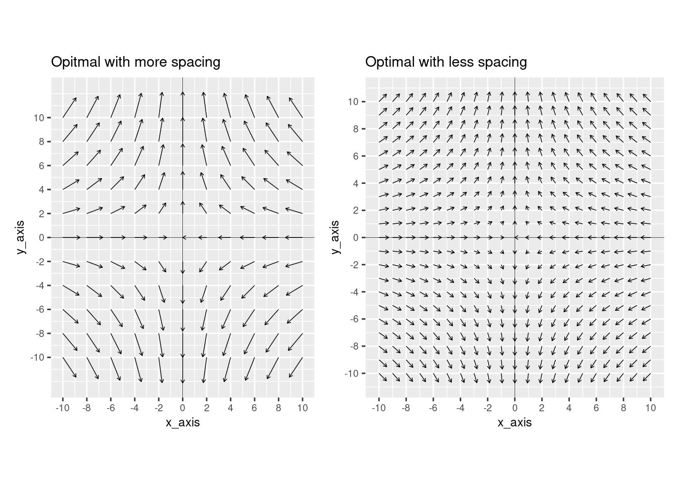

25.4 Dealing with 3D

So far we have looked at vector fields in 2 dimensions. However, it is common to for vector fields to have 3 dimensions. While it is tempting to try building 3D plots for these vector fields, we strongly recommend against as they are confusing. As shown in the plot below, which had been taken from this page.

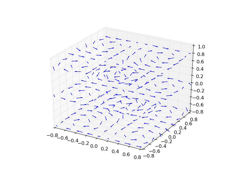
Therefore, the first thing to consider when plotting 3D vector fields should be: Do I actually need to plot in 3 dimensions?

In some cases, one dimension may have a small contribution to the overall flow, so it could be excluded from the plot. You could check this by comparing contributions of each direction to the magnitude of each vector using the following formulas x^2 / (x^2 + y^2 + z^2) , y^2 / (x^2 + y^2 + z^2) & z^2 / (x^2 + y^2 +z^2 ).

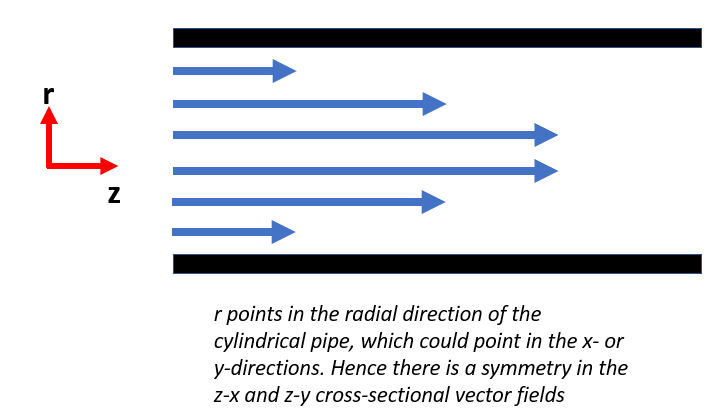
Another aspect to consider is the symmetry in the environment of the flow. For example, flow in a cylindrical is symmetric in any radial direction; in other words, if we say the flow is in the z-direction, cross-sectional flows will be identical in the z-x and z-y plots, see graph below for visual explanation.

If it is not possible to remove one axis due to its small contribution, or symmetry in the vector field, we recommend plotting 3 cross-sectional vector fields in the x-y, x-z and y-z planes. In this plot, the first thing to consider is where the cross-sections are taken from in the 3D space. We recommend cross-sections at the midpoint of each direction and adjusting the exact slices as appropriate. In the code below, we create a 3D vector field, show how to extract the midpoints of each axis, and plot vector fields at the cross-sections of these midpoints.

vector_frame = data.frame(x_axis = numeric(), y_axis = numeric(), z_axis = numeric()) 

# Generating a vector field in 3D space
for(i in -5:5) {
  for(j in -5:5) {
    for(k in -5:5) {
      vec <- c(i, j, k) 
      vector_frame[nrow(vector_frame) + 1, ] <- vec
    }
  }
}

vector_frame$x_pull <- with(vector_frame, -x_axis/(sqrt((x_axis^2) + (y_axis^2) + (z_axis^2) ) + 1))
vector_frame$y_pull <- with(vector_frame, y_axis/(sqrt((x_axis^2) + (y_axis^2) + (z_axis^2) ) ))
vector_frame$z_pull <- with(vector_frame, -z_axis/(sqrt((x_axis^2) + (y_axis^2) + (z_axis^2) ) +0.5))

# Finding midpoints of each axis
x_range <- range(vector_frame$x_axis)
mid_x <- (x_range[2] + x_range[1]) / 2

y_range <- range(vector_frame$x_axis)
mid_y <- (y_range[2] + y_range[1]) / 2

z_range <- range(vector_frame$z_axis)
mid_z <- (z_range[2] + z_range[1]) / 2

# Extracting each cross-section
xy_plot <- vector_frame[vector_frame$z_axis == mid_z,]
xz_plot <- vector_frame[vector_frame$y_axis == mid_y,]
yz_plot <- vector_frame[vector_frame$x_axis == mid_x,]

#Plotting the 3 cross-sections
xy <- ggplot(xy_plot, aes(x = x_axis, y = y_axis) )+
        scale_x_continuous(breaks = seq(-5,5,1)) + 
        scale_y_continuous(breaks = seq(-5,5,1)) +
        geom_segment(aes(xend = x_axis + (x_pull), 
                     yend = y_axis + (y_pull)), 
                     arrow = arrow(length = unit(0.1, "cm")), size = 0.25) +
        geom_vline(xintercept=0, size=0.15) + geom_hline(yintercept=0, size=0.15) +
        ggtitle("x-y cross-section") +
        coord_fixed() +
        theme(text=element_text(size=8))

xz <- ggplot(xz_plot, aes(x = x_axis, y = z_axis) )+
        scale_x_continuous(breaks = seq(-5,5,1)) + 
        scale_y_continuous(breaks = seq(-5,5,1)) +
        geom_segment(aes(xend = x_axis + (x_pull), 
                     yend = z_axis + (z_pull)), 
                     arrow = arrow(length = unit(0.1, "cm")), size = 0.25) +
        geom_vline(xintercept=0, size=0.15) + geom_hline(yintercept=0, size=0.15) +
        ggtitle("x-z cross-section") +
        coord_fixed() +
        theme(text=element_text(size=8))

yz <- ggplot(yz_plot, aes(x = y_axis, y = z_axis) )+
        scale_x_continuous(breaks = seq(-5,5,1)) + 
        scale_y_continuous(breaks = seq(-5,5,1)) +
        geom_segment(aes(xend = y_axis + (y_pull), 
                     yend = z_axis + (z_pull)), 
                     arrow = arrow(length = unit(0.1, "cm")), size = 0.25) +
        geom_vline(xintercept=0, size=0.15) + geom_hline(yintercept=0, size=0.15) +
        ggtitle("y-z cross-section") +
        coord_fixed() +
        theme(text=element_text(size=8))

xy + xz + yz + plot_layout(ncol=2)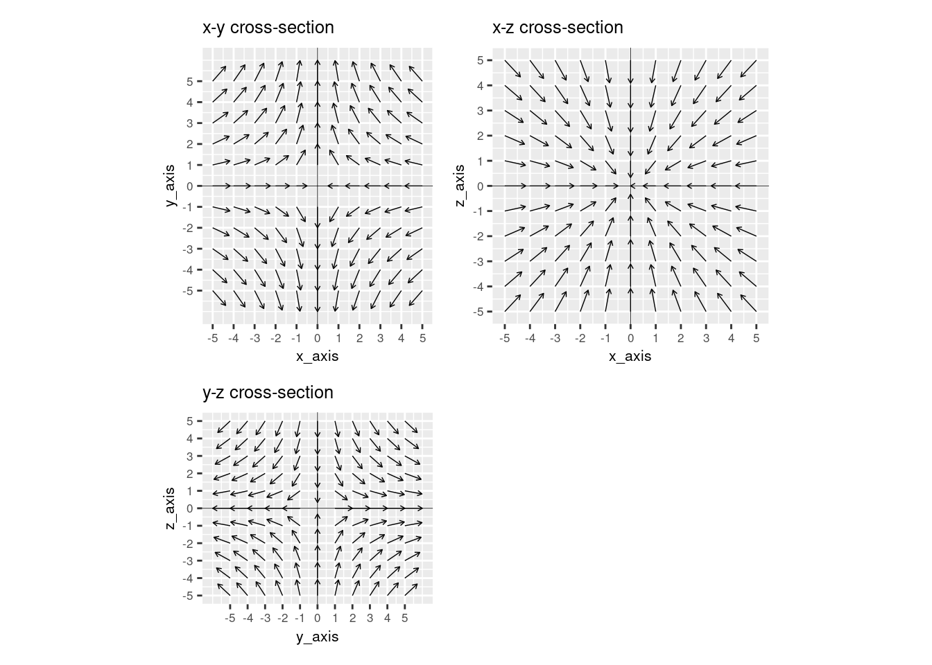

In summary, when visualizing 3D vector fields, you should avoid plotting in 3D. Instead, you should consider if one dimension has a small contribution and, if so, eliminate it from the plot. You should also think about whether symmetries in the vector field allow you to exclude a dimension from the plot. If neither option is possible, you should take cross-sections at the midpoints of the axes and plot the flows in 2D.

25.5 Application

Now that we’ve covered the fundamentals of plotting vector fields, we will briefly discuss some of their applications.

25.5.1 Flow

Using vector fields to visualize flow is extremely important in fluid mechanics. Examples of its application include:

Identifying regions of turbulence when designing airplanes or race cars
Discovering the sources and sinks of pressure fields in meteorology
Modelling flow through blood vessels with stents

25.5.2 Stability Analysis

Stability analysis models the long-term affects of small perturbations in initial conditions of dynamical systems. Using the differential equations that describe these environments, we can plot vector fields of the system and understand the nature of fixed points in the system (ie are the fixed points, stable, unstable, etc…). The figure below illustrates several types of fixed points:

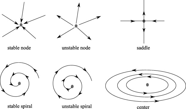
Source: https://www.sciencedirect.com/science/article/pii/S0021929018302239

Examples applications of stability analysis include modelling:

Firing rates in computational neuroscience
Gene regulation networks
Population dynamics

Therefore, given the differential equations describing the system, we can generate a data frame with the vectors at points in the environment. Then, using the skills learnt in this tutorial we can plot the vector fields, find the fixed points and determine their nature.

25.5.3 Conclusion

In this tutorial we have covered the following topics:

how to generate vector fields and adjust their components
the trade-off between arrow length and arrow spacing
methods of plotting vector fields with 3 dimensions
applications of vector fields in flow analysis and stability analysis

Using all of these tools, we hope the reader has a better understanding of how to construct vector fields, elements to consider when creating high-quality vector fields and where they could be applied in the real-world.

25.5.4 Reflection

From our research, there is limited documentation on plotting vector fields in R. Further, from resources that do exist, such as Vectorfield Recipe, we feel that the tutorial dives too deep too quickly. Therefore, our goal in this tutorial is to provide a clear, easily accessible introduction to building graphs of vector fields in R. Moreover, as engineering students who are familiar with vector fields, we wanted to share some advice on how to produce high-quality plots and briefly explain how these plots are used in research and development.

In all, we believe that we have successfully captured the basic principles in an accessible format for other readers and hope this tutorial contributes to a better understanding of vector fields in R. While we have had experience of plotting vector fields in Python, we have learned how to do so in R. We have also learned to explicitly express the elements to consider when plotting high-quality vector fields.

In terms of further work, we think it may have been useful to use actual vector field data sets, rather than only synthetically produced data, as it may provide the reader a more practical exposure to handling this data. Having said this, the majority of vector field data is simulated, so we believe this omission is not significant. Another area of further work could be to include illustrative tutorials walking the reader through how to produce vector field plots specific to flow analysis and stability analysis. However, we must be careful when making these additions as the analyses of these applications requires a deep knowledge of the topic, which could confuse the reader and fall into the trap of other tutorials that dive “too deep too quick”.

25.5.5 Extra

Overall, the motivation for our project was to provide a clear, easily accessible tutorial for building vector graphs. As engineering students, we have encountered vector graphs in many of our classes, but we found the existing documentation (Vectorfield Recipe) to be unnecessarily confusing, while also overlooking the basics of getting started. In all, we learned how to make vector graphs, and feel we successfully capture the basic principles in an accessible format for other readers. We don’t feel as if there are any major changes we’d make in improving the article.

24 googleVis in R

26 A Summary of Interactive Chart