36 Using raster data in R
Andre Evard
36.1 Introduction to rasters
This Community Contribution project gives an overview of the online book Geocomputation in R, specifically in regards to the raster type of geographic data representation. Please note, the second version of this book is in active development, so some packages and references may be out-of-date in the near future.
Frequent references to a package called terra are made, which may be read about in detail here. All extra data sources used here are detailed by the book, except this snow cover data that was found on a website, Zenodo, that Geocomputation in R already links to.
36.1.1 What is a Raster?
A raster is a spatial model that crosswise divides an area of land into regularized boxes, or cells. Each raster is strictly rectangular in the X and Y dimensions, each cell has the same dimensions and is defined by a point in one corner, and each stores associated values, say temperature, elevation, population density, the list goes on. A raster may have multiple layers, and each cell has exactly one value per layer.
These rasters are extremely useful for environmental scientific modeling outside of the confines of political boundaries, for example capturing the number of frog species discovered in square kilometer sections of the Amazon Rainforest, or they can be as widespread as the RGB pixels on the screen you are viewing this through.
For reference, the other type of geocomputational model the book is concerned about is the vector. It is defined by cells with specified shapes and geometries, which are better able to represent human political boundaries for instance. Although this project is centered on the raster, vectors will be referenced on occasion for data translation or transformation.
36.1.2 What is Terra?
(covers sections 2.3.1 through 2.3.3)
Terra is the primary package that Geocomputation with R cites for raster processing. Reportedly, terra is the more common usecase and easier to learn package, whilst stars’s niche is the premire for more specialized datasets. sf is the third and final package the book describes in heavy detail, but that is for vector data.
Terra is built upon the older raster package, with an internal foundation of C++ for efficiency. As for its Raster representation, in one of the book’s first code snippets, we can see its default attributes.
raster_filepath = system.file("raster/srtm.tif", package = "spDataLarge")
srtm = rast(raster_filepath)
As we can see here, the raster is defined by:
- dimensions:
- nrow: number of rows
- ncol: number of columns
- nlyr: number of layers
- resolution: the space to be covered by a single cell, in two dimensions
- extent: the boundaries of each coordinate
- coordinate reference: the distance’s data type (more about the “EPSG:4326” here)
And we have access to the additional fields of the source, name, class, and some small metadata.
terra also provides have dedicated functions to return the components:
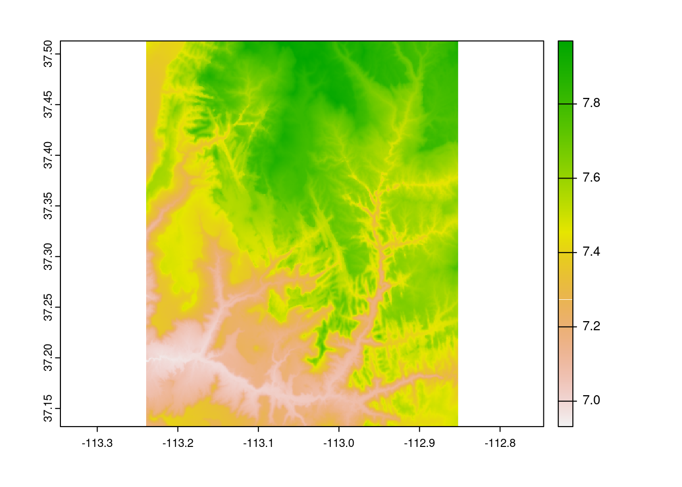
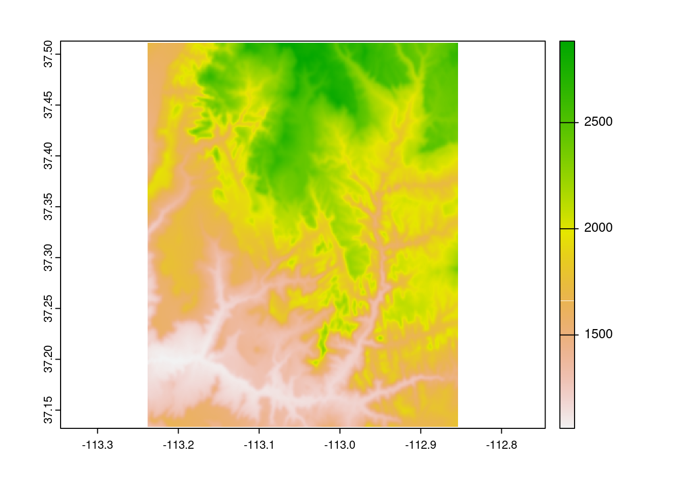
Geocomputation in R makes frequent usage of this example, srtm, an elevation map surrounding a Utah national park, and though we will provide other examples, sometimes its quick reference provides the best example. Quickly plotting it shows the following graphic:
plot(srtm)
And intuitively, each cell has its own value, represented visually through pixels by this color scale.
36.2 Raster Creation
36.2.1 The direct approach
(covers sections 2.3.4, and 3.3.1) So we know what rasters are, and a basic data structure. Okay, well how do we create, load, or populate more general rasters? There’s a few options, as always.
Naturally, we can directly create our own raster with the rast() function as follows:
manual_raster = rast(
  nrows = 100,
  ncols = 100,
  nlyrs = 2,
  resolution = .5,
  xmin = -25,
  xmax = 25,
  ymin = -25,
  ymax = 25,
  vals = 1:20000
)
plot(manual_raster)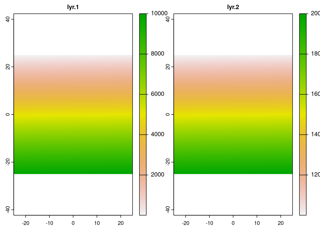
This isn’t exactly a terribly useful raster, but it is intuitive. You can also extract and replace these values, though those aren’t recommended for anything past small structures and experiments. With knowledge of what row/col values you’re targeting, you can directly set values in a similar fashion, using c() functions if more than one cell is desired. Mutliple layers may also be modified at a time this way. See the last section for a better approach to raster manipulation.
terra::extract(manual_raster, 10, 10)## lyr.1 lyr.2
## 1 10 10010
manual_raster[15, -10] <- 15000
manual_raster[15, -10]
## lyr.1 lyr.2
## 1 NA NA
manual_raster[c(19, 20, 21), c(19, 20, 21)] <- cbind(c(5000:5008), c(15000:15008))
plot(manual_raster)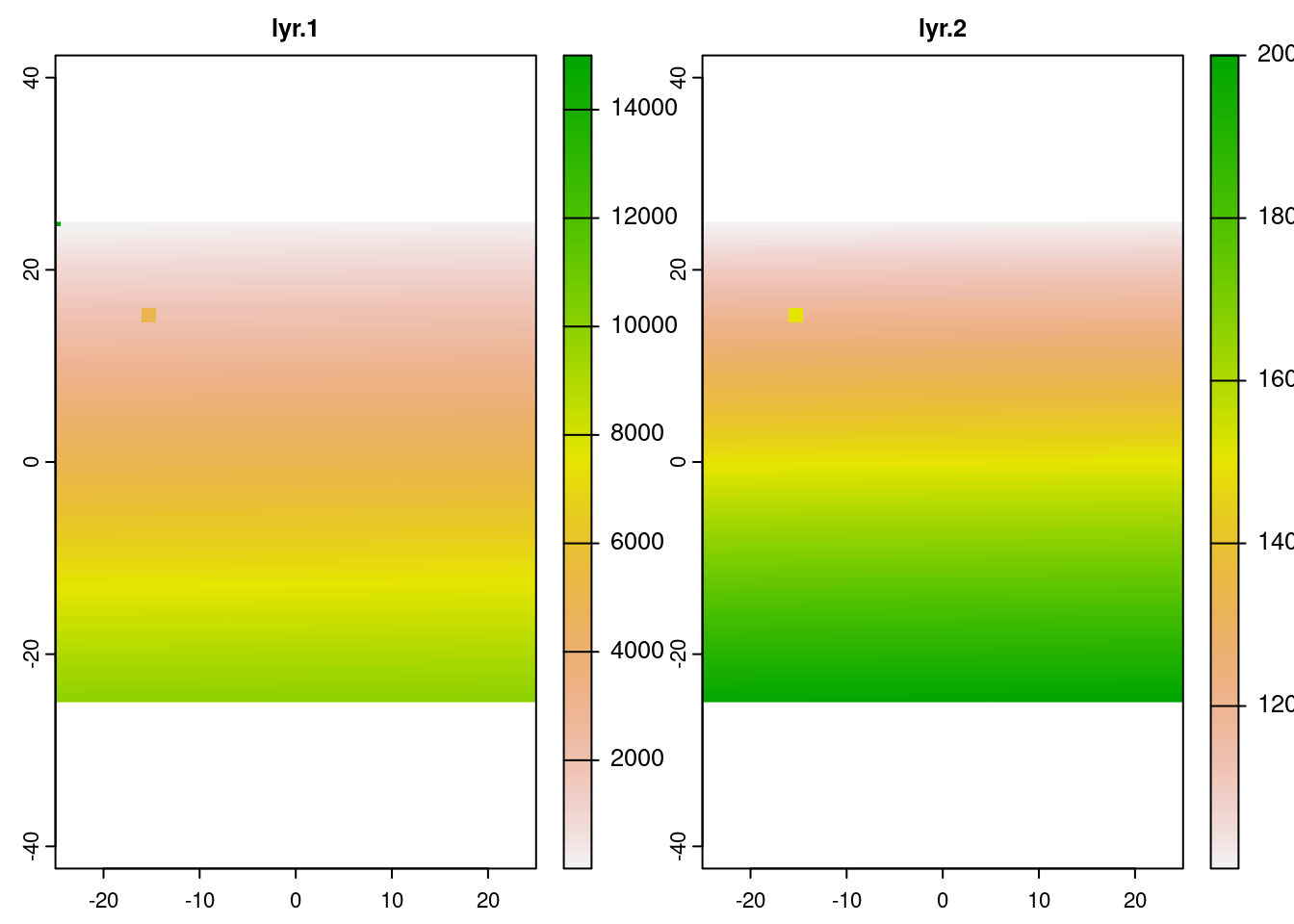
# You can also use <raster>[] as a shortcut of .values().36.2.2 Raster files and their formats
(covers sections 8.5 and 8.6.2)
Loading files is preferred approach and far more robust, should you have an image file already handy (or one you producedyourself!).
Firstly, there’s a lot to know about raster files. Pulling from section 8.5, we can find a quick overview of popular raster (and vector) formats. In short though, our primary file format will be GeoTIFF, which embeds additional geospatial data (such as coordinate systems) into .tif/.tiff image files. Among others, NASA and Google both have some of their data publicaly available as COGs.
Outside of GeoTIFF, there is also Arc ASCII (.asc) for text-based storage, SpatiaLite as an extension for SQLite, and ESRI FileGDB which is proprietary. So, outside of specific use cases, our recommendation is to use GeoTIFF.
Notably, GeoTIFF also supports Cloud Optimized GeoTIFFs (COG), which allows rasters to be hosted on HTTP servers and enables users to download only a segment of what can be rather large files.
Given a path, the rast() function does a good job at loading in rasters.
snowurl = "/vsicurl/https://zenodo.org/record/5774954/files/clm_snow.cover_esa.modis_p05_1km_s0..0cm_2001.01_epsg4326_v1.tif"
snow = rast(snowurl)
snow
## class : SpatRaster
## dimensions : 17924, 43200, 1 (nrow, ncol, nlyr)
## resolution : 0.008333333, 0.008333333 (x, y)
## extent : -180, 180, -61.99666, 87.37 (xmin, xmax, ymin, ymax)
## coord. ref. : lon/lat WGS 84 (EPSG:4326)
## source : clm_snow.cover_esa.modis_p05_1km_s0..0cm_2001.01_epsg4326_v1.tif
## name : clm_snow.cover_esa.modis_p05_1km_s0..0cm_2001.01_epsg4326_v1As previously mentioned, the whole GeoTIFF will not be downloaded at once this way, merely attached to. /vsicurl/ followed by the https url is all that’s necessary to download such information, provided you have the image provider located already of course. The relevant portions will be loaded if we utilize or manipulate it in some manner, such as this:
dimension_raster = rast(
  nrows = 1000,
  ncols = 1000,
  resolution = 0.008333333,
  xmin = 2.5,
  xmax = 17.5,
  ymin = 42.5,
  ymax = 57.5
)
snow_clipped = crop(snow, dimension_raster)
snow_clipped
## class : SpatRaster
## dimensions : 1800, 1800, 1 (nrow, ncol, nlyr)
## resolution : 0.008333333, 0.008333333 (x, y)
## extent : 2.499993, 17.49999, 42.50334, 57.50333 (xmin, xmax, ymin, ymax)
## coord. ref. : lon/lat WGS 84 (EPSG:4326)
## source : memory
## name : clm_snow.cover_esa.modis_p05_1km_s0..0cm_2001.01_epsg4326_v1
## min value : 0
## max value : 100
plot(snow_clipped, main="Snow cover around the Alps in Jan 2001")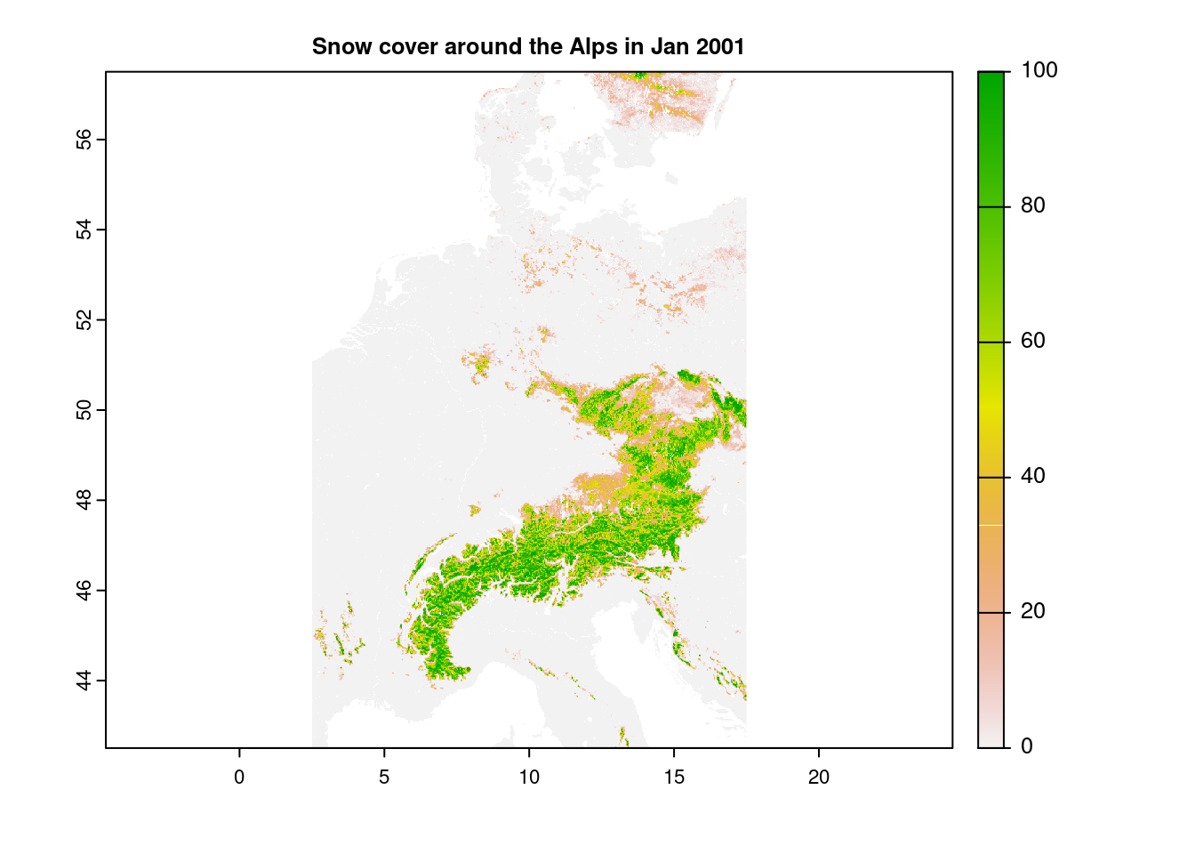
We will discuss cropping later. Naturally, we can also load local files using rast(). You can produce or save them yourself, or use packages such as spData.
# what it would look like with a local file
#snow_rast = rast("2019_jan_snow_cover.tif")
snow_rast = rast("/vsicurl/https://zenodo.org/record/5774954/files/clm_snow.cover_esa.modis_p95_1km_s0..0cm_2019.01_epsg4326_v1.tif?download=1")
USA_NE_raster = rast(
  nrows = 1000,
  ncols = 1000,
  resolution = 0.008333333,
  xmin = -83.5,
  xmax = -68.5,
  ymin = 35.5,
  ymax = 50.5
)
cropped_NE_snow = crop(snow_rast, USA_NE_raster)
plot(cropped_NE_snow, main="USA Northeast snow cover in jan 2019")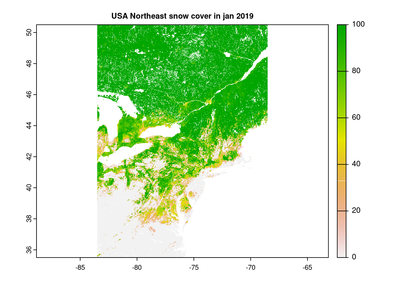
36.2.3 Rasterization
(covers section 6.4)
There’s one more type of raster creation: transformations from vectors, rasterize. Usage of these requires more knowledge of spatial vector data than we have time to go into depth here, but in short, it is a set of extremely flexible operations that convert various statistics from a vector set and transform that into some sort of grid. Examples provided are state boundaries, aggregating the count or average values of point clusters, and we’re confident that with the right vector datasets the possibilities are quite endless.
More at Geocomputation with R’s section 6.4 if you’re curious.
36.3 Raster Manipulations, and their applications
So knowing how to create them is all well and good, but what can we do with rasters? How do we use them?
36.3.0.1 Spatial operations
There are a good number of geometrically-based operations that terra supports out of the box. The sections that Geocomputation with R lays out are Subsetting in 4.3.1, Local, Focal, Zonal, and Global map algebra operations in sections 4.3.3 through 4.3.6, and raster Merging in section 4.3.8
36.3.1 Subsetting
(covers section 4.3.1)
There are a few ways to (cleanly) draw values from individual cells, the cells, rows, or columns ids from coordinates, or to slice apart the data. cellFromXY() and assorted functions, and terra::extract are two good ones, though beware the overlap with tidyverse’s extract. We can also define smaller rasters and clip or crop them through, as we have done in examples prior.
xy <- matrix(c(-73.94, 40.73), ncol = 2)
matrix_cells = cellFromXY(cropped_NE_snow, xy)
cropped_NE_snow[matrix_cells]
## clm_snow.cover_esa.modis_p95_1km_s0..0cm_2019.01_epsg4326_v1
## 1 31
terra::extract(cropped_NE_snow, xy)## clm_snow.cover_esa.modis_p95_1km_s0..0cm_2019.01_epsg4326_v1
## 1 31
filter = rast(
  xmin = -74.5,
  xmax = -73.5,
  ymin = 40.2,
  ymax = 41.2,
  resolution = 0.0083
)

NYC_sieve = terra::extract(cropped_NE_snow, ext(filter))
head(NYC_sieve)
## clm_snow.cover_esa.modis_p95_1km_s0..0cm_2019.01_epsg4326_v1
## 1 62
## 2 61
## 3 68
## 4 74
## 5 75
## 6 81
# extract does a lot more things more flexibly, cellfromxy and related
# better for method header precision and location manipulation
# NYC was not very snowy that winter, it seems...
As well as direct access, should we know either the desired row & column numbers or the 1D cell ids:
srtm[50, 50]## srtm
## 1 1885## srtm
## 1 1854
## 2 1919
## 3 1986
## 4 1835
## 5 1885
## 6 1962
## 7 1819
## 8 1869
## 9 1929
srtm[100]## srtm
## 1 203436.3.2 Cropping and Masking
(covers section 6.2)
Two similar concepts, crop() and mask() perform the task of downsizing a raster, typically in tandem, and both require the usage of an additional spatial object, in practice typically a vector. Where they differ is that cropping reduces the dimensions of the original raster based on the second object’s boundaries, whereas masking sets everything outside of the second object’s boundaries to zero, but leaves the structure intact.
zion = read_sf(system.file("vector/zion.gpkg", package = "spDataLarge"))
zion = st_transform(zion, crs(srtm))
srtm_cropped = crop(srtm, zion)
srtm_masked = mask(srtm, zion)
plot(zion[0], main="Outline of Zion national park")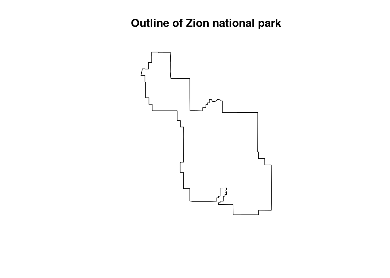
plot(srtm_cropped, main="SRTM cropped by Zion national park")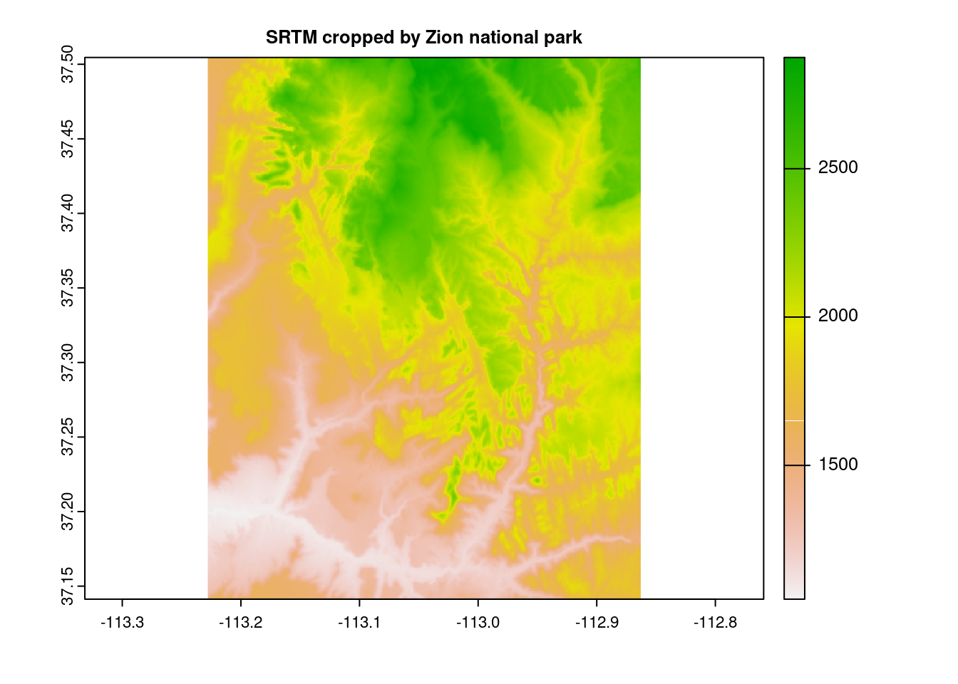
plot(srtm_masked, main="SRTM masked by Zion national park")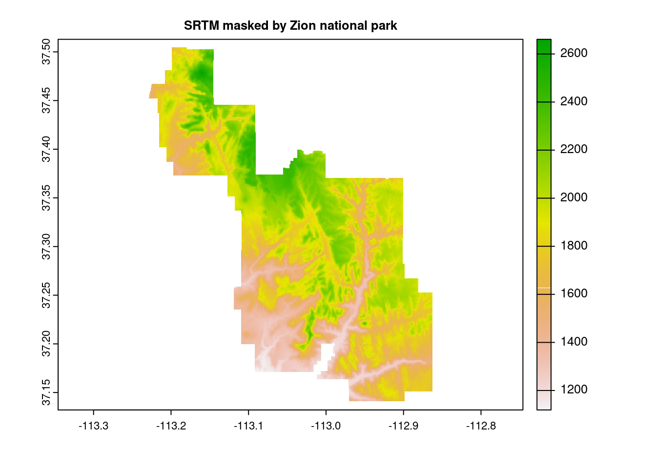
And of course we can combine them:
plot(crop(srtm_masked, zion))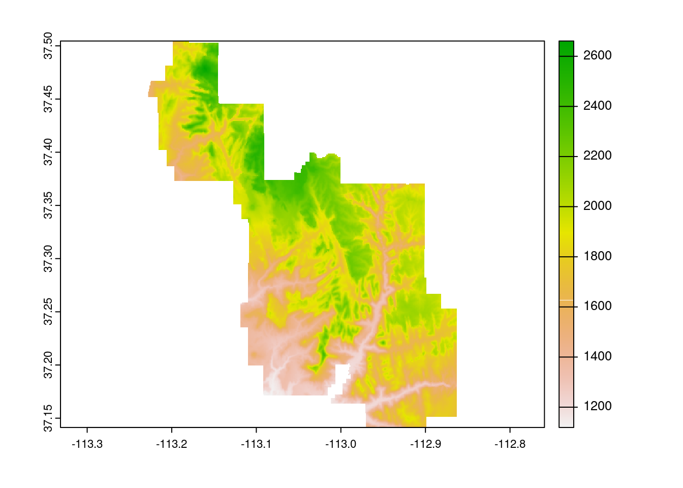
36.3.3 Map Algebra
(covers sections 4.3.2, 4.3.3, 4.3.4, 4.3.5, and 4.3.6)
As we can see here, many algebraic calculations can be performed on rasters at the local level.
srtm = rast(system.file("raster/srtm.tif", package = "spDataLarge"))
plot(srtm)
plot(srtm ^ 2)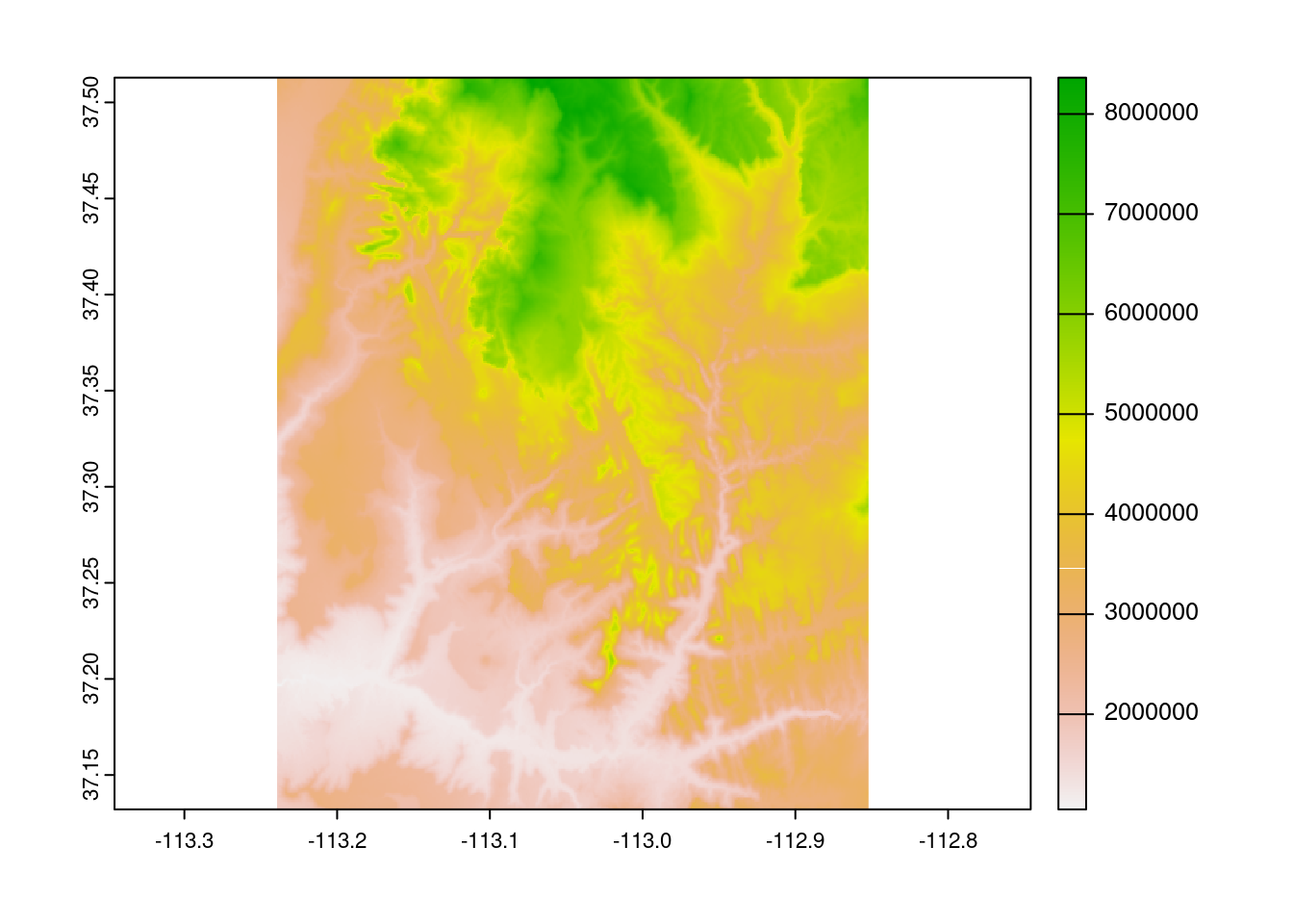
As well as boolean operations
plot(snow_clipped > 20, main="Areas with more than 20% snow cover")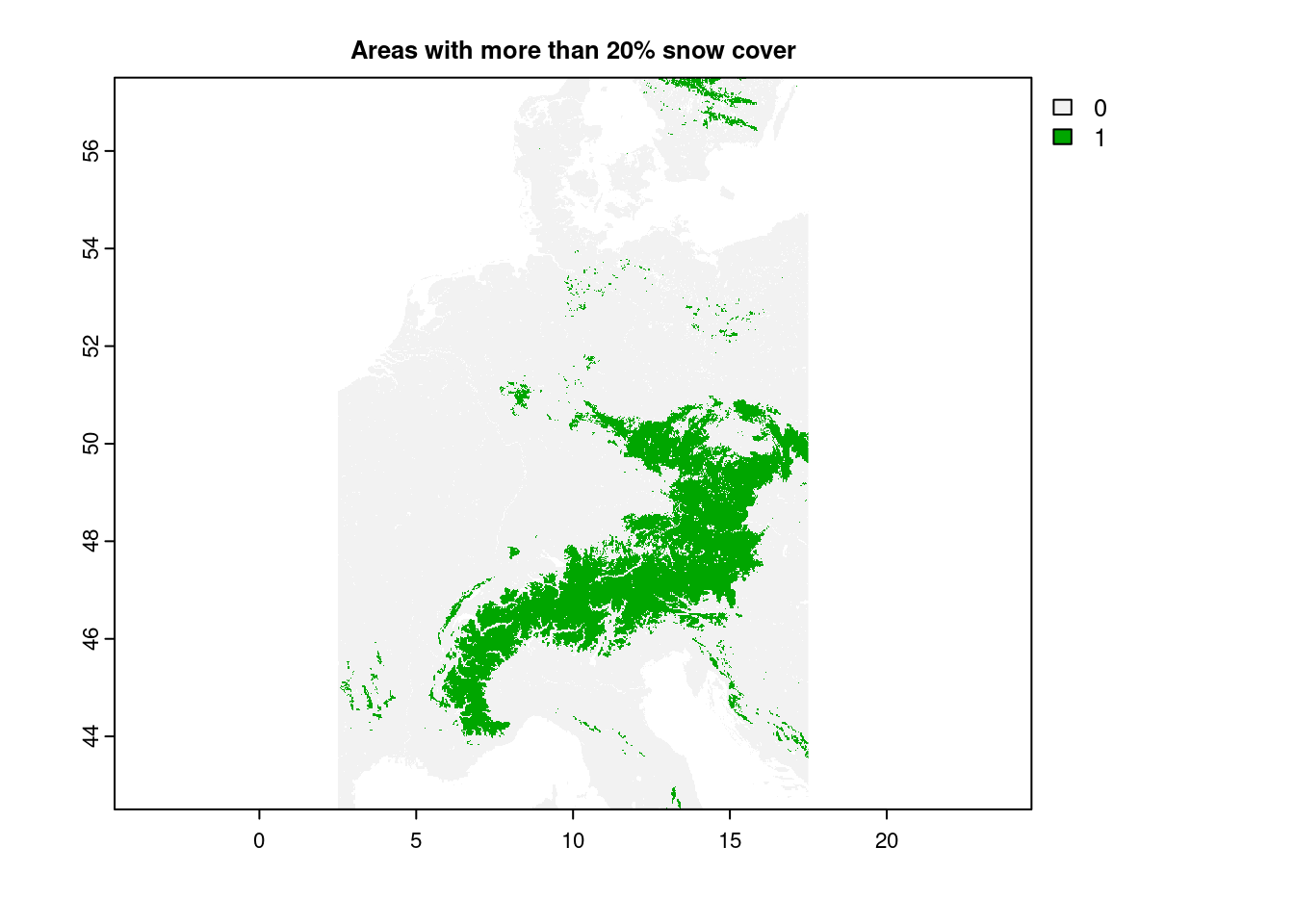
plot(snow_clipped == 0, main="Areas with no snow cover")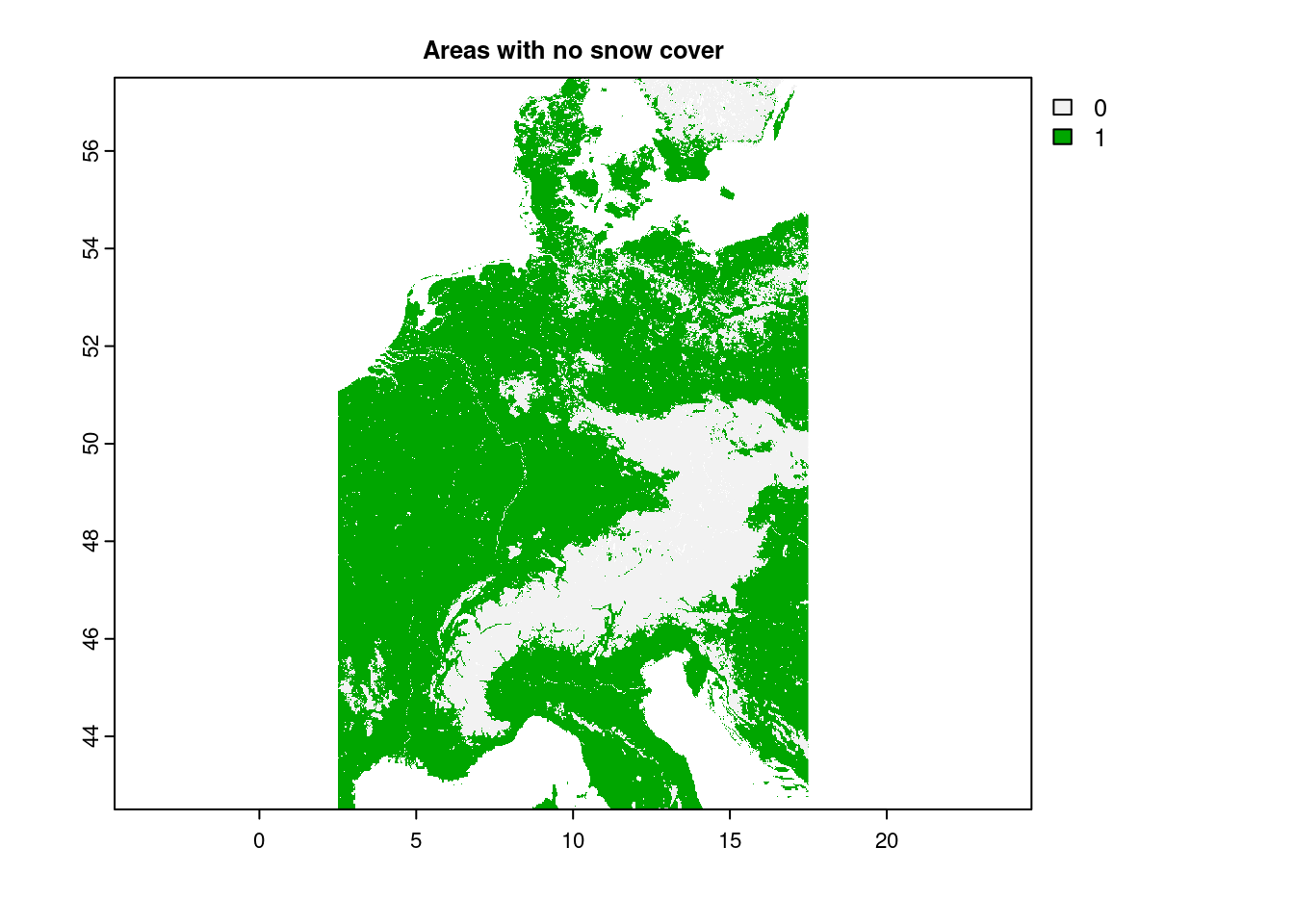
And through the use of app() for efficiency on large data.
app(snow_clipped, fun=function(i) { 2 * log(i) })## class : SpatRaster
## dimensions : 1800, 1800, 1 (nrow, ncol, nlyr)
## resolution : 0.008333333, 0.008333333 (x, y)
## extent : 2.499993, 17.49999, 42.50334, 57.50333 (xmin, xmax, ymin, ymax)
## coord. ref. : lon/lat WGS 84 (EPSG:4326)
## source : memory
## name : lyr.1
## min value : - ?
## max value : 9.21034Given the right attributes in the data (the book lists coil class, pH, etc), this can be used for predictive modeling.
Focal transformations:
Similar to sliding windows in some machine learning algorithms, focal operations transform cells by their neighborhoods, working to process out extremes whilst preserving the form of the original data. Another potential focal operator is terrain(), which calculates terrain characteristics from elevation data.
Zonal is similar to focal but one level of aggregation up. It uses a second raster to define zones to group the first by, applying statistical measurements on that divided population.
Global are cross-raster statistical calculations, and can be used for distance and a few other possibilities–namely, summary functions we’d see on any type of dataset.
summary() describes the archetypal statistical bands, freq() counts the occurrences of each class, and boxplot(), density(), hist(), and pairs() can all be run out-of-the-box for immediate exploration. global() remains the most robust approach, as you can self-define a statistical function yourself to apply your particular dataset, much as you can with the aforementioned app() and its entourage.
summary(snow_clipped) # 3rd quartile of 1, but mean of 10?## clm_snow.cover_esa.modis_p05_1km_s0..0cm_2001.01_epsg4326_v1
## Min. : 0.00
## 1st Qu.: 0.00
## Median : 0.00
## Mean : 10.27
## 3rd Qu.: 1.00
## Max. :100.00
## NA's :28886
snow_tenths = app(snow_clipped, fun=function(i) {ceiling(i / 10) * 10})
freq(snow_tenths) # Indeed, 0 is by far the most common
## layer value count
## 1 1 0 1696965
## 2 1 10 190843
## 3 1 20 61456
## 4 1 30 44132
## 5 1 40 42039
## 6 1 50 43384
## 7 1 60 46092
## 8 1 70 47859
## 9 1 80 46767
## 10 1 90 43627
## 11 1 100 4677236.3.4 Extraction
(covers section 6.3)
Extraction is the process of gathering a targetted subset of values from a raster, through the use of terra::extract(). It will take the use of vector spatial objects, but the result is some rather powerful if specialized inferences. We’ll keep it brief, but please visit 6.3 if you’re interested further.
Example use cases of raster extraction can vary as wildly as your creativity. For a few quick examples, we could import the boundaries of European country around the alps and aggregate snow cover there, or find the highest/lowest points along Zion National Park’s boundaries. The demonstrations the book provides are picking elevation from a selection of points, and the elevation graph along a line segment for planning a hike. Categorical and continuous data can both be extracted, sometimes at once across different layers.
One quick note–the book points out there can be performance issues at scale, and to use exact_extract() from the exactextract package where possible.
36.3.5 Vectorization
(covers section 6.5)
The opposite of rasterization, spatial vectorization transforms rasters into vectors. If you’re familiar with vectors, there is again an abundance of flexibility here, lying in the as.spatvector class of functions. One particularly eye-catching use is the quick visualization of contour lines using as.contour() as follows:
cl = as.contour(srtm)
plot(cl, axes=FALSE)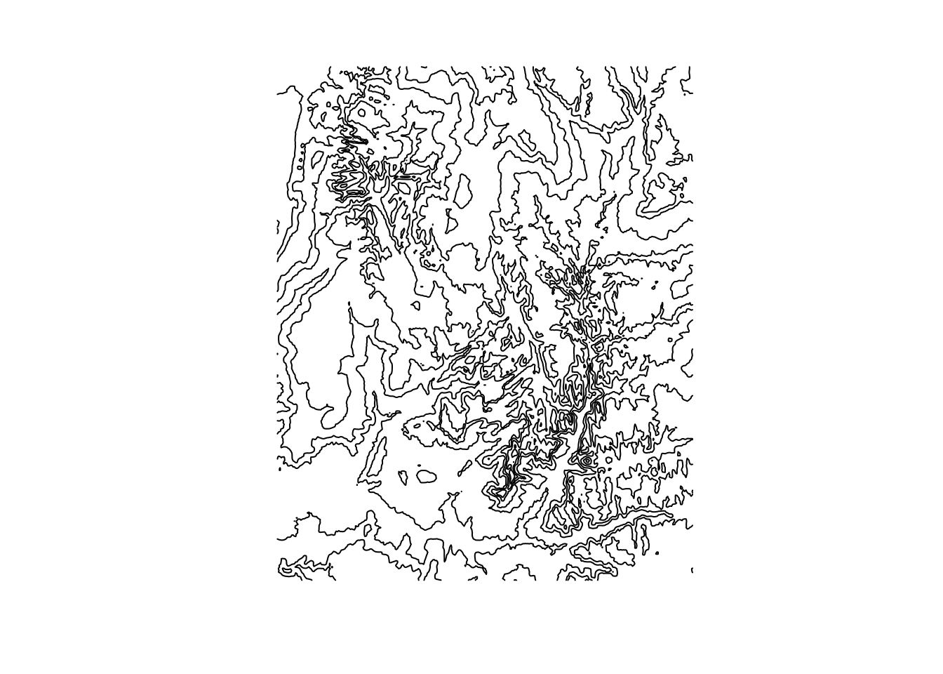
36.3.6 File Output
(covers section 8.7.2) Okay, so you’ve done your experiments, and would like to preserve your rasters to share your results and save on later computational power. How?
Simple. writeRaster().
# Is how I would do it, if I wanted to dirty the CC project
# writeRaster(snow_clipped, filename="2007_jan_eu_snow.tif", datatype="INT1U",
#             overwrite=TRUE)
There is a little more involved, such as selecting the bit datatype for storage, filetypes if writeRaster can’t infer it from the filename, names for the layer names, and an assortment of memory-related variables for debugging and throughput of particularly large rasters. Compared to loading in rasters, though, this function is conveniently straightforward, yet still plenty capable in terms of flexibility; like rasters as a hole, rigid, yet surprisingly flexible just one layer beyond the surface.