23 How to use sqldf

Conor Ryan

library(sqldf)
library(tidyverse)

23.1 Motivation

sqldf is a library that lets you work with dataframes as if they were database tables, such that you can query them and do whatever SQL-style manipulation you want, without worrying about the logistics of managing any databases. It can be useful for various dataframe manipulations, as we often need to do when preparing data for visualization.

There are a few reasons why I thought the library could use a tutorial:

• Its Github page is kind of a mess, and its official CRAN documentation is not particularly user-friendly.
• This is a pretty cool tool when you think about it: with no overhead or extra work, we can just call SQL on a dataframe.
• The option to use SQL is incredibly useful when dealing with working in many languages. If I need a quick R visualization but was just working with Python, it might be easier to just manipulate my data via SQL rather than figure out the exact R syntax that would do the same thing.
• Certain data manipulation is just more suited for SQL syntax, like complicated left joins and window functions.
• When the scale of our data gets too large for memory, this library offers some impressive advantages. Even if you can load the large dataset into memory, doing so will be slow; it is way faster to do your initial manipulation (like filtering the data down 100-fold) through this library, after which it is more reasonable to deal with the resulting dataframe.
• This approach is a significant improvement over something like dbplyr and the knitr SQL engine. Such an approach still requires manual management of connections and tables. Additionally, knitr is hardly suited for non-report-style work in R. sqldf is usable in a wider variety of scenarios.

23.2 Usage

23.2.1 Basics

Once you’ve installed the sqldf, it really is as easy as loading the library and writing some SQL:

sqldf('select * from iris') |> head()

##   Sepal.Length Sepal.Width Petal.Length Petal.Width Species
## 1          5.1         3.5          1.4         0.2  setosa
## 2          4.9         3.0          1.4         0.2  setosa
## 3          4.7         3.2          1.3         0.2  setosa
## 4          4.6         3.1          1.5         0.2  setosa
## 5          5.0         3.6          1.4         0.2  setosa
## 6          5.4         3.9          1.7         0.4  setosa

We did not have to create any database, load our data to any table, or cleanup the table. The package handled it all behind the scenes.

We can do some more realistic, basic manipulation. In R we might do:

iris |>
  filter(Petal.Length > 2.0) |>
  mutate(Sepal_Product = Sepal.Length * Sepal.Width) |>
  group_by(Species) |>
  summarize(mean_sepal_product=mean(Sepal_Product)) |>
  head()

## # A tibble: 2 × 2
##   Species    mean_sepal_product
##   <fct>                   <dbl>
## 1 versicolor               16.5
## 2 virginica                19.7

While in SQL we can do:

sqldf('
  select Species, avg(`Sepal.Length` * `Sepal.Width`) as mean_sepal_product
  from iris
  where `Petal.Length` > 2.0
  group by 1
') |>
  head()

##      Species mean_sepal_product
## 1 versicolor            16.5262
## 2  virginica            19.6846

23.2.2 More advanced SQL tasks

This library becomes more powerful as you use it to do things SQL is uniquely good at. For example, although a simple join on a matching column condition is relatively easy in R (and Python), the following sort of condition is more annoying to accomplish:

sqldf('
  select a.Species, b.Species, avg(a.`Sepal.Width`) as `a.Width.Avg`
  from iris a
  join iris b
    on a.species != b.species
    and a.`Sepal.Length` > b.`Sepal.Length`
    and a.`Sepal.Width` < b.`Sepal.Width`
  group by 1,2
') |>
  head()

##      Species    Species a.Width.Avg
## 1 versicolor     setosa    2.764037
## 2 versicolor  virginica    2.738889
## 3  virginica     setosa    2.901931
## 4  virginica versicolor    2.737284

Similarly, window functions become far more accessible through this package:

sqldf('
  select Species, avg(`Sepal.Length`) over (partition by Species order by `Sepal.Length` desc rows between unbounded preceding and current row) as running_mean
  from iris
') |>
  head()

##   Species running_mean
## 1  setosa     5.800000
## 2  setosa     5.750000
## 3  setosa     5.733333
## 4  setosa     5.675000
## 5  setosa     5.640000
## 6  setosa     5.600000

These are unique tasks where it might even be preferable to just use SQL rather than the R dataframe manipulation. Which is fine; not every tool can do everything prefectly – SQL excels at very specific things.

23.2.3 Alternate data sources

We also don’t have to already have the dataframe in-memory to use this library. Suppose iris was in a .csv on our machine:

# disabled because we were asked to not write any data
write.table(iris, 'iris.csv', sep = ",", quote = FALSE, row.names = FALSE)

and we wanted to immediately get it into memory with a few rows filtered out:

# disabled because we were asked to not write any data
read.csv.sql('iris.csv',  sql = 'select * from file where "Petal.Length" > 2.0') |>
  head()

This is great because we didn’t ever have to have the “useless” version of the dataframe ever in our code; immediately we get this version that has some filtering done.

Or, what if the data lives as a .csv on some remote host?

read.csv.sql(
  'https://gist.githubusercontent.com/netj/8836201/raw/6f9306ad21398ea43cba4f7d537619d0e07d5ae3/iris.csv',
  sql = 'select * from file where "Petal.Length" > 2.0'
) |>
  head()

##   sepal.length sepal.width petal.length petal.width      variety
## 1          7.0         3.2          4.7         1.4 "Versicolor"
## 2          6.4         3.2          4.5         1.5 "Versicolor"
## 3          6.9         3.1          4.9         1.5 "Versicolor"
## 4          5.5         2.3          4.0         1.3 "Versicolor"
## 5          6.5         2.8          4.6         1.5 "Versicolor"
## 6          5.7         2.8          4.5         1.3 "Versicolor"

Hopefully you can see why these options are powerful. Although iris is small, sometimes our data is very large, and we may not want to deal with loading many millions of rows into R if we are going to filter it down anyway. There is an example of this later under the Performance section.

23.2.4 Advanced database usage

Under the hood, sqldf actually loads each dataframe into a temporary database table. If we want, we can also manage the database more intelligently. This is a more contrived use case, but worth knowing. Suppose you’re dealing with a lot of data and plan to do two subsequent queries. It would be better to only read the dataframe into a table once and reuse that table. This can be accomplished via:

sqldf() # keep iris as a table in the db

## <SQLiteConnection>
##   Path: :memory:
##   Extensions: TRUE

sqldf('select * from iris') |> # iris now loaded as a table. can reuse it.
  head()

##   Sepal.Length Sepal.Width Petal.Length Petal.Width Species
## 1          5.1         3.5          1.4         0.2  setosa
## 2          4.9         3.0          1.4         0.2  setosa
## 3          4.7         3.2          1.3         0.2  setosa
## 4          4.6         3.1          1.5         0.2  setosa
## 5          5.0         3.6          1.4         0.2  setosa
## 6          5.4         3.9          1.7         0.4  setosa

sqldf() # connection closed and iris table deleted

## NULL

You can also just pass any database administrative command to the above function as well. For example, you could manage the entire database (create new schemas, tables, adjust permissions) if you really wanted to. Although doing so in a more appropriate tool might be worth considering.

23.3 Performance

Certain tasks actually end up more optimal if done through sqldf. For example, the following arbitrarily large join, which fans out to nearly a billion rows, took roughly 30 seconds on my laptop to finish. (Although the below task is nonsense, in real data, one may come across a use case that actually needs to do something similar.)

sqldf('
  select count(*)
  from iris a
  join iris b using (species)
  join iris c using (species)
  join iris d using (species)
  join iris e using (species)
')

##    count(*)
## 1 937500000

The following R equivalent, which only does the third ‘join’, took longer than all four took in SQL. To preserve my computer, I did not attempt the fourth merge below (commented out).

merge(iris, iris, by="Species") |>
  merge(iris, by="Species") |>
  merge(iris, by="Species") |>
  #merge(iris, by="Species") |>
  nrow()

## [1] 18750000

This library also becomes helpful when dealing with large datasets on disk. For example, the below arbitrary .csv was ~600MB (I did not include the file with this project, but feel free to try it with your own large file). Because the below does not require we load the entire file into R first, it finished in about 30 seconds.

# disabled because I cannot provide this (intentionally) large file
read.csv.sql(
  '~/Downloads/star2002-1.csv',
  sql='select `X1`, avg(`X807`) from file where `X4518` > 5500 group by 1'
) |>
  head()

This is a worthwhile improvement; the below R equivalent completed in 45 seconds.

# disabled because I cannot provide this (intentionally) large file
read.csv(file = '~/Downloads/star2002-1.csv') |>
  filter(X4518 > 5500) |>
  group_by(X1) |>
  summarize(some_avg=mean(X807)) |>
  head()

This difference becomes more meaningful as your dataset’s size increases relative to your machine’s memory. Once the file is several GB, preprocessing in a temporary database table becomes increasingly more efficient relative to pure R. We observed a marginal version of this optimization above. This functionality is especially useful if we know we will never need to refer back to the full file (meaning we will only use e.g. the transformed version as above).

23.4 Combining with ggplot

We can also combine sqldf manipulations with ggplot to easily make visualizations. When we use sqldf in the scenarios it excels at, as outlined above, this becomes powerful. There are infinite combinations here, so here is one simple illustrative example:

sqldf('
      select Species, avg(`Sepal.Width`) as avg_width
      from iris
      group by 1
') |>
  ggplot(aes(x=reorder(Species, avg_width), y=avg_width)) +
  geom_bar(stat='identity') +
  coord_flip() +
  xlab('Species')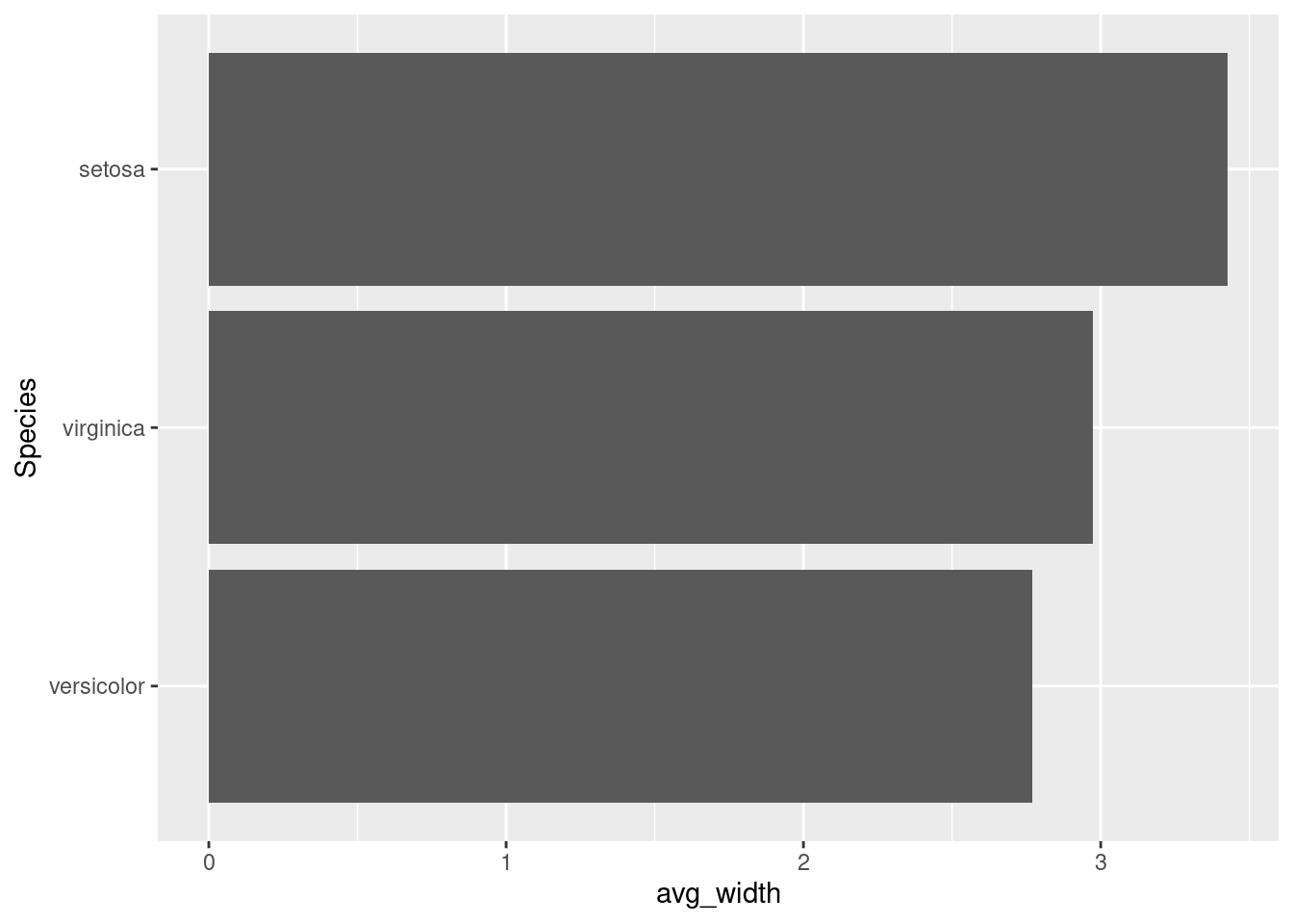

23.5 Conclusion

sqldf is an important option to have available when manipulating data. To be clear, it is not a replacement for knowing how to use R in general. One should restrict themselves to using sqldf only when doing so is uniquely advantageous to SQL-style work, or if they don’t want to deal with writing perfect R. The above guide should be useful to anyone new to the library as to exactly which scenarios one might opt to use it in.

Personally, I’m glad I chose to do a deep dive into this library and create this guide. It was educational in many ways, like: learning more about databases, understanding how R can blend with SQL, and elucidating the things that R vs. SQL each excel at. I will certainly be be referring back to this document, as I think it makes it easy to review exactly how to quickly use the library, without getting too in-the-weeds of all its nuts and bolts (as much of its existing documentation does, in my opinion). One thing I’d like to dedicate more effort to next time is exactly replicating complex SQL commands in R; knowing how to do so will likely be useful at some point, even if not practical right now. Finally, I wish I had known about this library sooner, as I know that it will for sure optimize parts of my workflow going foward.

23.6 References

https://github.com/ggrothendieck/sqldf

https://cran.r-project.org/web/packages/sqldf/index.html

https://www.geeksforgeeks.org/window-functions-in-sql/