Chapter 67 Chinese translation links

Some groups of students have contributed to the community by translating useful resources into another language.

67.1 R and ggplot2

Yuchen Pei and Jiaqi Tang

We translated two online tutorials for visualizaiton in R into Chinese. The first one is called A Comprehensive Guide to Data Visualization in R for Beginners and the second one is called ggplot2: Mastering the basics. Our translation files can be found here: https://github.com/Jasmine1231/EDAV-19Fall-Community_Contribution .

67.2 forcats package

Xu Xu and Xiaoyun Zhu

引言：

说到数据分析，我们不得不提大神 Hadley Wickham。

Hadley Wickham 是 RStudio 的首席科学家以及 Stanford University, Rice University 统计系的兼职教授。他是著名图形可视化软件包 ggplot2 的开发者，以及其他许多被广泛使用的软件包的作者，代表作品如 plyr、reshape2 等。

Wickham曾说过：“通过数据从根本上了解世界真的是一件非常，非常酷的事情”，而整理数据正是透过数据看世界的第一步。作为一个多产的R开发者，Wickham乐于给那些喜欢摆弄数据的人提供力量和支持。他就创建了一个便于整理分类数据(categorical data)的包forcats，用于处理因子，可以更高效地对因子进行修改。

下面我们翻译了一篇R-bloggers上讲解forcats用法的文章（作者是S.Richter-Walsh)，希望这个教程可以让大家在整理数据时更得心应手。

这是原文链接，供大家参考：https://www.r-bloggers.com/cats-are-great-and-so-is-the-forcats-r-package/

翻译正文：

Forcats是由Hadley Wickham创建的一个做数据整理时非常好用的包。在进行数据分析和建模之前，我们经常需要花大量的时间来清理数据（或者说预处理数据）。要我估计的话，我认为一个数据科学家会花至少70%-80%的时间来清理数据。这也是学校所教和业界真实项目之间最大的区别。学校教学时所用的数据集经常是预处理过后整齐的数据，但实际工作中的数据集基本不可能是这样的。我很喜欢清理数据，并喜欢分析在清理过程中出现的问题。我发现forcats这个包在整理分类数据时非常有效。

67.2.1 示范数据准备

我们用下面的代码生成一些数据用于示范。这个数据集是关于销售数据的，其中有50个缺失数据(NA), 7个因子。

library(dplyr) # Also load up dplyr so we can use the pipe operator: %>%
library(forcats)

df <- data_frame(sales = factor(rep(c("Online",
 "Post",
 "Web",
 "Call Centre",
 "Inbound Phone",
 "Outbound Phone",
 "Field Sales",
 NA), 50)),
 buy = sample(c(0, 1), 400, replace = T)) %>%
 mutate(sales = sample(sales, size = length(sales), replace = T))

table(df$sales)

## 
##    Call Centre    Field Sales  Inbound Phone         Online Outbound Phone 
##             49             47             57             41             48 
##           Post            Web 
##             61             53

67.2.2 关于缺失数据(NAs)的处理

缺失数据在实际工作中很常见。在R的数据框(dataframe)中计算连续变量的均值(mean)，中位数(median)，方差(variance)和标准差(standard deviation)时，我们需要考虑这些缺失数据。另外，如果我们希望用某个数据集来建模，我们也需要处理缺失数据来保留某些特定的变量和防止数据的缺失。我们常用的策略有用均值或中位数来代替连续型数据中的缺失值或用众数来代替分类数据中的缺失值。但有些情况下这些策略并不可取，我们有时需要将缺失数据设为一个明确的因子水平。我们可以通过forcats::fct_explicit_na()来实现这个目标，而且只需要一行代码。下面就让我们在示范数据上尝试一下：

df$sales <- fct_explicit_na(df$sales)

table(df$sales)

## 
##    Call Centre    Field Sales  Inbound Phone         Online Outbound Phone 
##             49             47             57             41             48 
##           Post            Web      (Missing) 
##             61             53             44

通过上面的处理，现在缺失数据都由一个明确的因子来表示，之前的缺失数值直接由(Missing)来代替。我们还可以用下面的代码来给这个新的因子命名：

df$sales <- fct_explicit_na(df$sales, na_level = "My New Level")

67.2.3 同义因子水平

有时分类变量会包含两个及更多指向同一分组的因子水平。语法表示可能会有细微差别，比如以大写字母开头和以小写字母开头（GroupA vs. groupA）。在这种情况下，我们可以用 forcats::fct_collapse() 来合并多个同义分子水平到一个里。在我们的测试数据中，让我们假设Web和Online指向同一销售渠道。我们想要合并这两个成为一个名为Online的因子水平。

df$sales <- fct_collapse(df$sales, Online=c("Online", "Web"))

67.2.4 混合多个频率低的因子水平成为一个

另一种可能发生的情况是，我们想使用需要大的样本容量来维持统计显著性的数据群组进行分析或者建模。设想一个因子变量有20个水平，但是只有其中的5个能用来解释数据集中90%以上的观测值。你可以全部剔除这些观测值，但是如果可能，要尽量避免数据丢失。或者，你可以混合多个频率低的因子水平成为一个覆盖它们全部的水平，在保持其余的和这些观测值相关的属性变量不变的同时整理了群组水平。这个函数混合多个频率低的水平成为一个名为Other的默认水平，并且保持这个水平中的数据数量为全部水平中最小的数量。使用者还可以用n参数来调整混合之后所保留的水平数量。在我们的测试数据中，名为Outbound，Phone 的水平是频率最低的，所以它们被混合进了一个新的名为Other的水平中。

df$sales <- fct_lump(df$sales)

67.2.5 在ggplot2 条形图中改变条的顺序

tidyverse是一系列包含dplyr，ggplot2，和forcats的包。这个包为数据科学家们创造了一个完美的工具生态系统。我想要介绍一下forcats::fct_infreq() 函数。这个函数可以在探索性数据分析和数据展示的阶段与ggplot2一同使用。有时改变条形图中因子的顺序可能有些难办，但是使用forcats包可以使这个任务简单化。

library(ggplot2)
ggplot(df, aes(x = fct_infreq(sales))) + geom_bar()

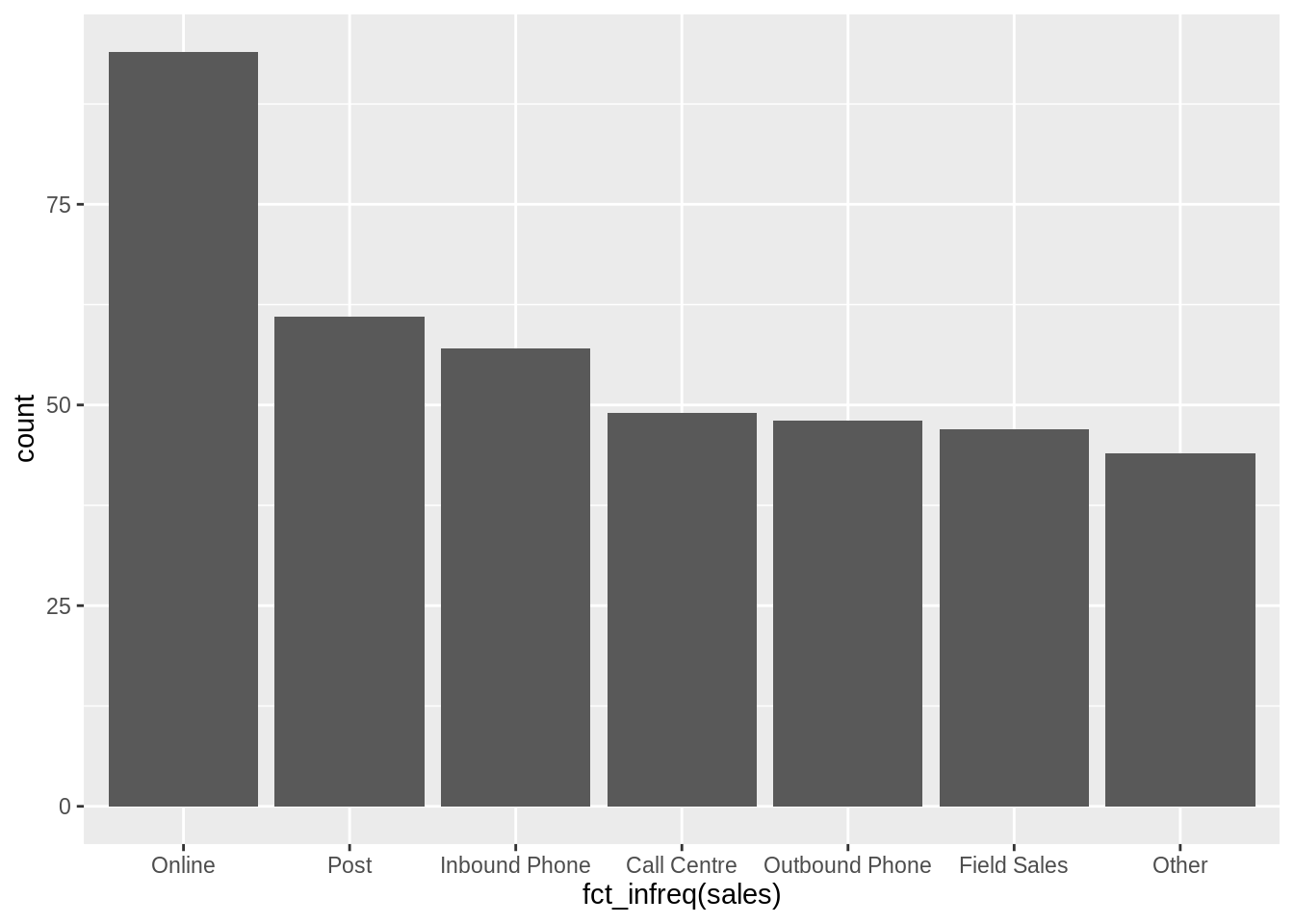
现在因子水平按照频率递减的顺序排列好了，并且包含了（缺失的）和Other。通过使用forcats来进行一些快速的预处理，我们没有丢失任何原数据。祝大家天天开心！

67.3 Continuous variables with R (Chinese)

Bangwei Zhou and Zhihao Ai

We created a tutorial in Chinese on the content of continuous variables with R. We combined (and translated) texts from chapter three of the textbook Graphical Data Analysis with R by Antony Unwin and the Continuous Variables section on edav.info. Additionally, we also included an example to better illustrate how a user can fully utilize R to assess continuous variables from PSET1 problem 1.

We hope this document can effectively jumpstart any user (with limited language background to Chinese) with sufficient skills to assess continuous variables with R.

Our document can be found here.

67.4 Visualising Spatial Data

Mutian Wang and Siyuan Wang

We translated a tutorial Introduction to Visualising Spatial Data in R written by Robin Lovelace, James Cheshire, Rachel Oldroyd. The source text can be found here.

Our translation can be found on our GitHub repo. In this repo, you can see our translation in the html file, and the source code in the Rmd file.