Chapter 50 Rmarkdown tutorial
Author: Shaofeng Wu, Mingrui Liu
50.1 1. Overview
R Markdown provides a tidy framework for data science. A markdown file can normally help us:
- save and execute code that you wrote
- generate high quality reports that can be shared with an audience
R Markdown documents are fully reproducible and support dozens of static and dynamic output formats.
This link provide a quick tour of what’s possible with R markdown.-links
50.1.1 1.1 What is R Markdown?
- Rmd files
· An R Markdown(.Rmd) file is a record of your project. It contains the code that your audience needs to reproduce your work as well as all the scripts that your audience can understand what you did.
- Reproducible Research
· You can useKnitto rerun the code in an R Markdown file to reproduce your work and export the results to be a well-formatted report.
- Dynamic Documents
· There are a lot of ways to export your report. The formats include html, pdf, MS Word, or RTF documents; html or pdf based slides, Notebooks, and more.
50.1.2 1.2 Workflow
- Open a new .Rmd file at File ▶ New File ▶ R Markdown.
- Write document by editing template
- Knit document to create report; use knit button or
render() to knit
- Preview Output in IDE window
- Publish (optional) to web server
- Examine build log in R Markdown console
- Use output file that is saved along side .Rmd

50.2 2. Getting started
50.2.1 2.1. Install the package
You can use the following command to install the required library.
50.2.2 2.2. Open file
You can create a new file or open existed from the directory that you choose.
50.2.3 2.3. output format
The Rmarkdown can render any Rmd file into a format that Rmarkdown supports. For example, the code below renders OutputExample.Rmd to a Microsoft Word document.
library(rmarkdown)
render("resources/rmarkdown_tutorial/OutputExample.Rmd", output_format = "word_document")
Following is a table of all the formats that you can choose: Output value table
| output value | creates |
|---|---|
| html_document | html |
| pdf_document | pdf (requires Tex ) |
| word_document | Microsof Word (.docx) |
| odt_document | OpenDocument Text |
| rtf_document | Rich Text Format |
| md_document | Markdown |
| github_document | Github compatible markdown |
| ioslides_presentation | ioslides HTML slides |
| slidy_presentation | slidy HTML slides |
| beamer_presentation | Beamer pdf slides (requires Tex) |
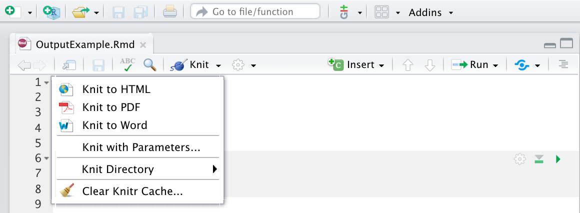
You can choose to render to the format that you want by clicking the dropdown menu beside the knit button:

50.3 3. Markdown syntax
Rmarkdown has lots of fancy syntax so that you can produce an ordered and beautiful document.
We will give the syntax here that we regularly use a lot.
plain text
plain text- italics and bold
*italics* and **bold**italics and bold
- list
* unordered list
   + sub-item 1
   + sub-item 2
- sub-sub-item 1 - unordered list
- sub-item 1
- sub-item 2
- sub-sub-item 1
1. ordered list
2. item 2
 i) sub-item 1
A. sub-sub-item 1 - ordered list
- item 2
- sub-item 1
A. sub-sub-item 1
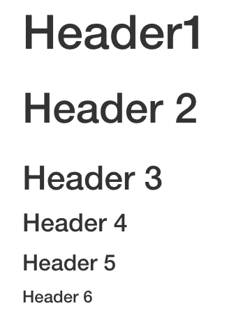
- headers
# Header1 {#anchor}
## Header 2 {#css_id}
### Header 3 {.css_class}
#### Header 4
##### Header 5
###### Header 6 
Caption
- hyperlink
<http://www.rstudio.com>
[link](www.rstudio.com)
Jump to [Header 1](#anchor)
http://www.rstudio.com link Jump to Header 1
- table
| Right | Left | Default | Center |
|------:|:-----|---------|:------:|
| 12    | 12   | 12      | 12     |
| 123   | 123  | 123     | 123    |
| 1 | 1 | 1 | 1 | | Right | Left | Default | Center |
|---|---|---|---|
| 12 | 12 | 12 | 12 |
| 123 | 123 | 123 | 123 |
| 1 | 1 | 1 | 1 |
- equation
$$E = mc^{2}$$ \[E = mc^{2}\]
50.4 4. Embeding code
50.4.1 4.1. Inline code
You can surround code with back ticks and r. R will replace inline code with its results.
For example:
The output is:
one plus one equals 2
50.4.2 4.2. Code chunks
In this way, ou need to start a chunk with ``` {r} and end a chunk with ```
For example:
## [1] "Hello, world!"50.4.3 4.3. Display options
There are also a lot of options to display your codes and results.
For example, you can choose eval as TRUE or False in the output to decide whether to evaluate the code and include its results.
Here is the difference between the two options:
With eval = TRUE:
## [1] "Hi there!"With eval = FALSE:
Here is a table that includes the options that we normally use:
| option | default | effect |
|---|---|---|
| eval | TRUE | Whether to evaluate the code and include its results |
| echo | TRUE | Whether to display code along with its results |
| warning | TRUE | Whether to display warnings |
| error | FALSE | Whether to display errors |
| message | TRUE | Whether to display messages |
| tidy | FALSE | Whether to reformat code in a tidy way when displaying it |
| cache | FALSE | Whether to cache results for future renders |
| comment | “##” | Comment character to preface results with |
50.5 5. Rendering
first way
You can run
rmarkdown::render("<file path>")in the console.second way
You can click the
Knitbutton in the top pane and choose the output format that you want.