Chapter 15 Fluctuation plots

Arusha Kelkar and Tanvi Pareek

Visualization involves using graphics to display and interpret the data to reveal the information in the dataset in a better sense. Fluctuation plots are one of the great ways to visualize data.

Fluctuation plots are used to visualize categorical data. It is a plot consisting of rectangles aligned next to each other where the number of rectangles depends on the number of categories in the data. Every position in the grid of the fluctuation plot represents a combination of categories in the data. The frequency of combinations of categories determine the relative sizes of the rectangular plots. Each rectangular plot has a foreground and a background. The background rectangle represents the maximum of all the frequencies for all combinations of categories in the data. The foreground rectangle represents the frequency of that particular combination of categories. So, the size of the foreground rectangle is relative to the maximum value of the frequencies.

Before giving an example of this using a dataset, we would like to outline the steps for the installation of the package extracat (archived in CRAN) which is used for plotting fluctuation plots in R.

Download the latest tar file from the following link https://cran.r-project.org/src/contrib/Archive/extracat/
If you don’t have the TSP package installed then download it by typing the following command in the R console install.packages(“TSP”, dependencies = TRUE).
In the terminal type the following command to install the extracat package: R CMD INSTALL -1 C:/Users/User/Desktop/Fluctuation extracat_1.7-6.tar

Make sure the path where the package is downloaded is correct.

Now we’re ready to plot the fluctuation plots in R!

We have used the HairEyeColor dataset which is already available in R. It gives the distribution of hair and eye color and sex in 592 students. The library extracat is loaded first and then the dataset.

library(extracat)
HairEyeColor

## , , Sex = Male
## 
##        Eye
## Hair    Brown Blue Hazel Green
##   Black    32   11    10     3
##   Brown    53   50    25    15
##   Red      10   10     7     7
##   Blond     3   30     5     8
## 
## , , Sex = Female
## 
##        Eye
## Hair    Brown Blue Hazel Green
##   Black    36    9     5     2
##   Brown    66   34    29    14
##   Red      16    7     7     7
##   Blond     4   64     5     8

The above output gives two tables separated based on the sex as Female or Male. Basically this is found by cross tabulating 592 values on 3 variables. The variable Hair has four levels namely Black, Brown, Red and Blond and the variable Eye has four levels namely brown, blue, hazel and green.

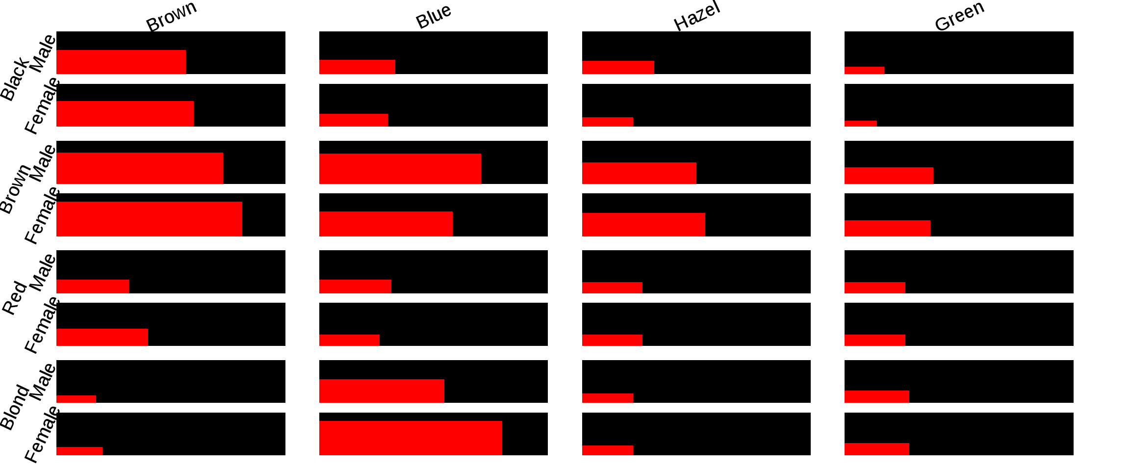
The function used to plot the fluctation diagrams is fluctile.

fluctile(HairEyeColor)

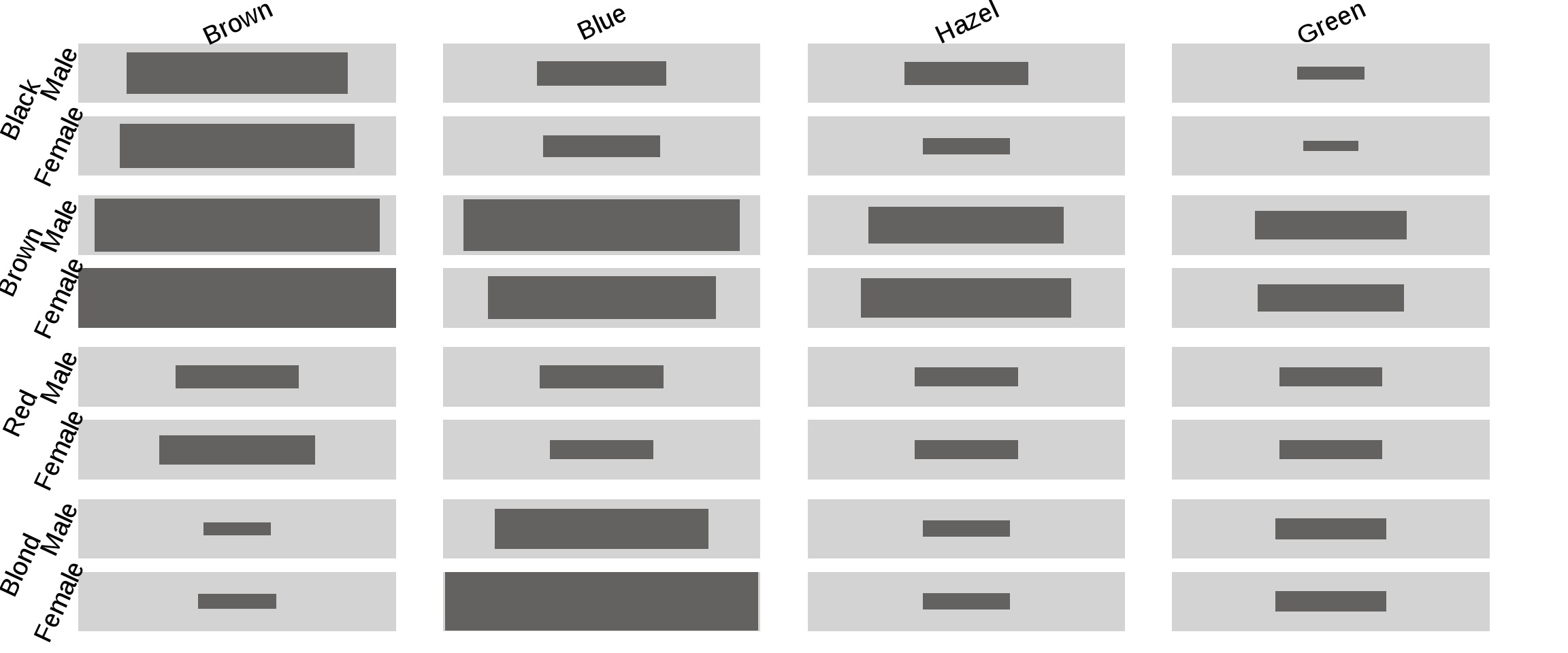
The default is that the rectangles are centered. We can change this default by using the just argument. tile.col is used to change the foreground colour and bg.col is used to change the background colour.

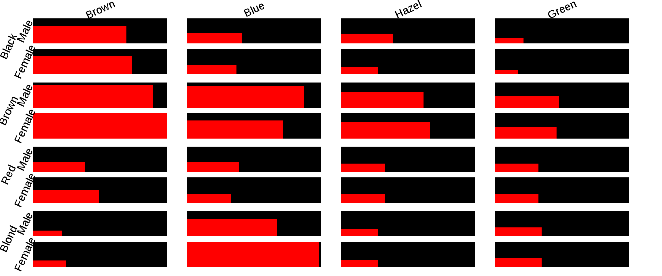
fluctile(HairEyeColor, just = "lb", tile.col = "red", bg.col = "black")

This leftbottom representation is more easy to interpret than the centred one.

The frequency in the dataset for entries with Brown hair, brown eyes and the person is female is the highest i.e 66.Therefore in the above plot, the foreground rectangle for these values of the categories covers the background rectangle completely. The maximum size of this background rectangle which is colored black is due to the maximum frequency i.e. the frequency of people being female,having brown hair and brown eyes which is 66.

All the other values, which are the counts of the values of the combinations of the 3 variables used here, are plotted with respect to this value.For example, the number of females having red hair and brown eyes is 16, so the proportion here is 16/66 , so that proportion of the rectangle is colored red.

Variations in plot:

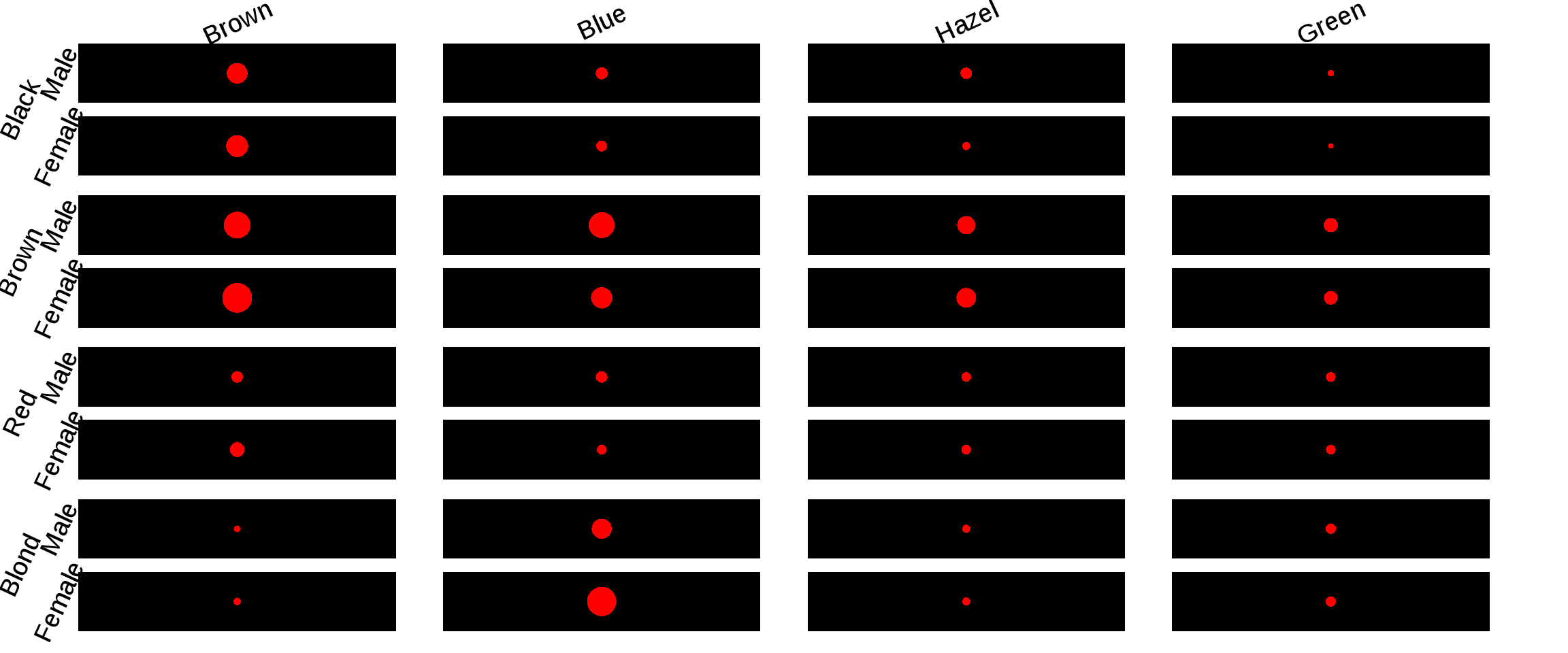
The shape of the plot below has been changed to circle using shape argument.

fluctile(HairEyeColor,shape="c", tile.col = "red", bg.col = "black")

The shape of the plot below has been changed to octagon using shape argument.

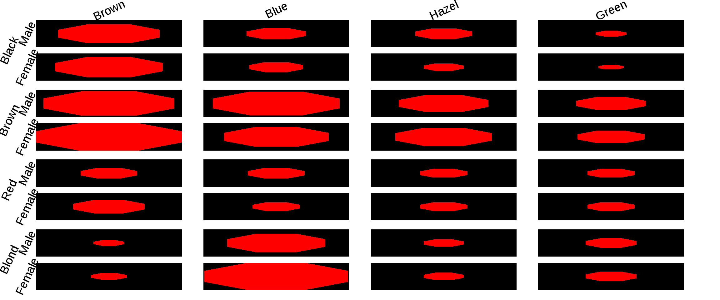
fluctile(HairEyeColor,shape="o",tile.col = "red", bg.col = "black")

The above 2 plots are variations of the rectangular fluctuation plots.These also give the insights about the frequencies of the combinations of categories at a glance.

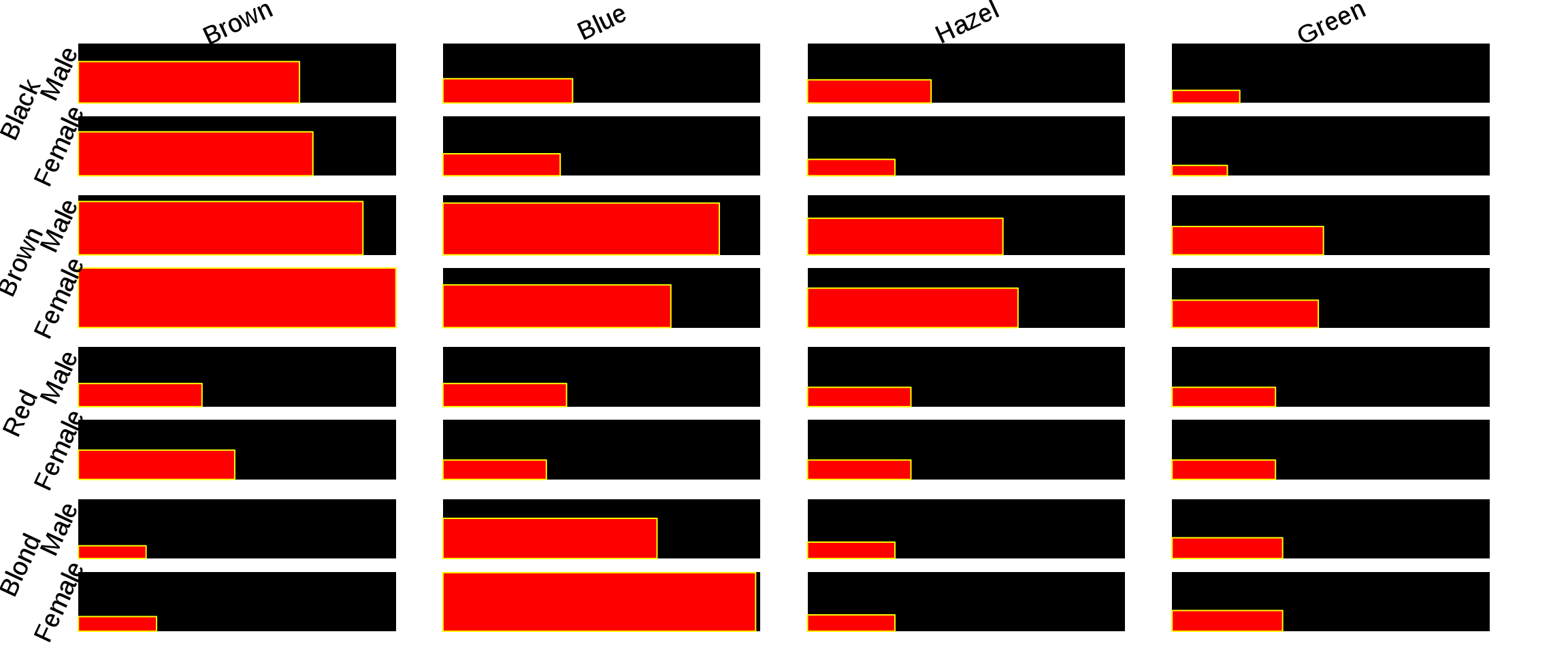
If you want to change the maximum value(the background) relative to which the foreground is plotted, you can set it using maxv argument. For example, below we have set maxv = 100 .

fluctile(HairEyeColor,just = "lb" ,tile.col = "red", bg.col = "black" , maxv = 100)

For adding border to the foreground, use the tile.border argument.

fluctile(HairEyeColor,just = "lb" ,tile.col = "red", bg.col = "black" ,tile.border = "yellow")

Why Fluctuation Plots?

This plot is very helpful for comparing frequencies of combinations of categories with the maximum of these frequencies.

Fluctuation diagrams are good for representing large contingency tables or transition matrices, where there is no reason to differentiate between the row variable and the column variable.

If there is a large number of combinations and only a few occur at all,then a fluctuation diagram is valuable for revealing this information and for identifying categorical clusters.