Chapter 48 Time Series Modeling with ARIMA in R
William Yu
This document will give a brief introduction to time series modeling with ARIMA in R. A time series is a set of data points that are indexed by time order. Time series modeling is an especially important topic in data analytics and data science because of its important applications towards various topics. This includes predicting the next day price of a stock, or patterns in the weather.
An important concept in time series modeling is ARIMA, or Auto-Regressive Integrated Moving Average. ARIMA is the combination of two models, the auto-regressive and the moving average models. An auto regressive AR(p) component refers to the use of past values in the regression equation for the series Y. The auto-regressive parameter p specifies the number of lags, or past values, to be used in the model. For example, AR(2) is represented as
\[Y_t = c + \phi_1y_{t-1} + \phi_2 y_{t-2}+ e_t\]
where φ1, φ2 are parameters for the model. The moving average nature of the model is represented by the “q” value, which is the number of lagged values of the error term. A moving average MA(q) component represents the error of the model as a combination of previous error terms et. The order q determines the number of terms to include in the model
\[Y_t = c + \theta_1 e_{t-1} + \theta_2 e_{t-2} +...+ \theta_q e_{t-q}+ e_t\]
Together, with the differencing variable d, which is used to remove the trend and convert a non-stationary time series to a stationary one, these three parameters define the ARIMA model. Thus, ARIMA is specified by three order parameters: (p, d, q).
ARIMA modeling boils down to five parts:
- Visualize the time series
- Stationarize the time series
- Plot ACF/PACF and find optimal parameters
- Build the ARIMA model
- Make predictions.
This document will provide information for all five. Let’s get started.
48.1 1. Visualize the time series
We’ll attempt to predict stock returns by using ARIMA. We’ll be using some financial data from tidyquant:
# get historical data for single stock. e.g. google
library(tidyquant)
jnj = tq_get("JNJ", get="stock.prices", from="1997-01-01") %>%
  tq_transmute(mutate_fun=to.period,period="months")
Let’s say we are primarily interested in the closing prices of our stock:
library(ggplot2)
# showing monthly return for single stock
ggplot(jnj, aes(date, close)) + geom_line()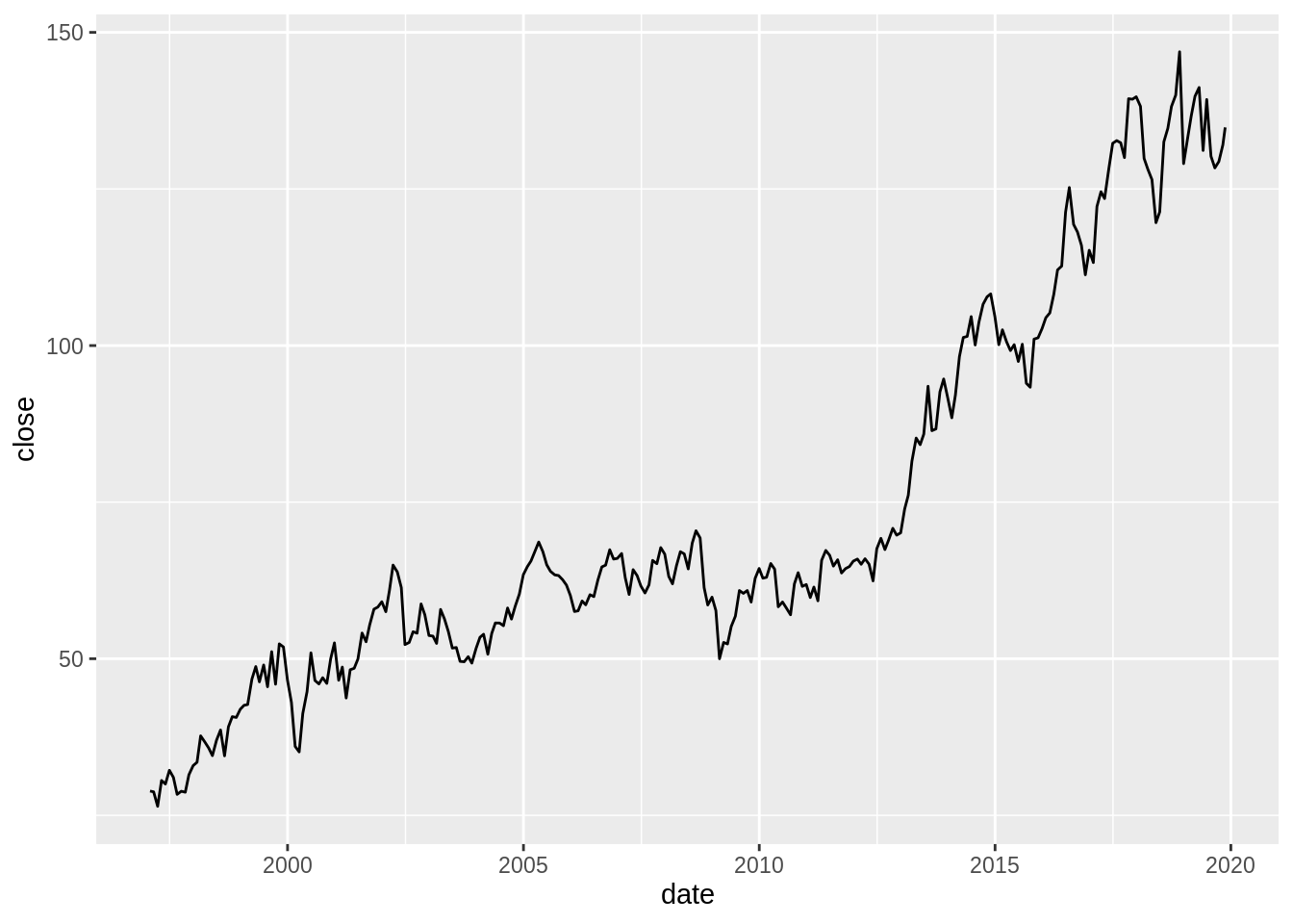
We are interested in predicting the returns of JNJ. We compute the log difference of the closing price to stationarize the time series. More on this in the next section.
48.2 2. Stationarize the Time Series
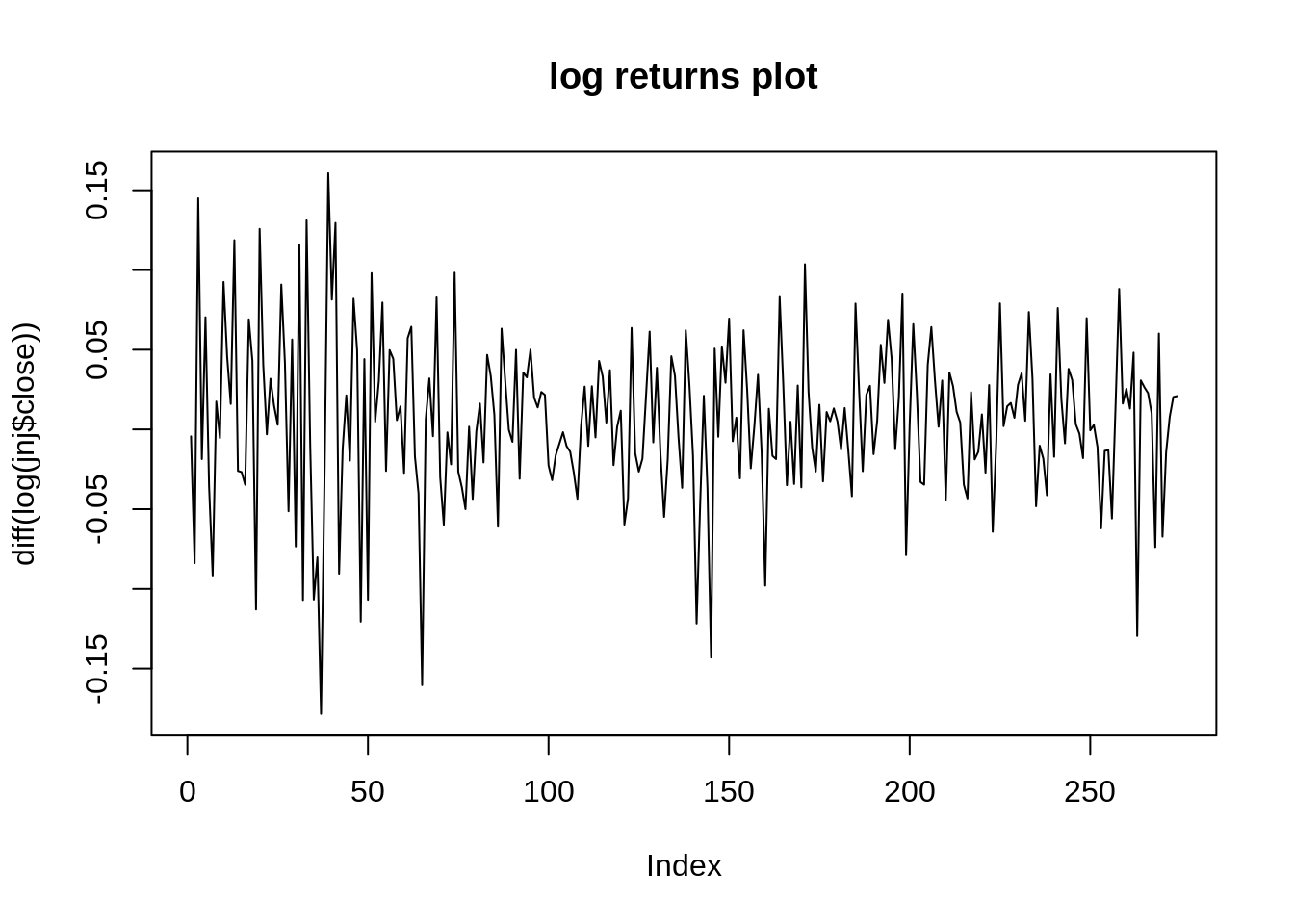
In order to perform any successive modeling on our time series, our time series must be stationary: that is, the mean, variance, and covariance of the series should all be constant with time. Now, there are many reasons as to why we must have a stationary time series, but probably the most important fact as to why we need this is because we literally cannot model a time series any other way; if the mean, variance and covariance vary with time, how will we actually be able to estimate our desired parameter?
Returns look stationary in the plot above. Let’s double check with the Dickey Fuller Test of Stationarity:
##
##  Augmented Dickey-Fuller Test
##
## data:  diff(log(jnj$close))
## Dickey-Fuller = -17.966, Lag order = 0, p-value = 0.01
## alternative hypothesis: stationary
The Dickey-Fuller test returns a p-value of 0.01, resulting in the rejection of the null hypothesis and accepting the alternate, that the data is stationary.
It is quite common in financial analysis to predict stock returns. By taking the difference between stocks, we are essentially stationarizing the time series. Though not all stock returns are stationary, in many experiments regarding financial analysis, many assume it is.
48.3 3. ACF/PACF
ACF stands for Auto-Correlation Function. ACF gives us values of any auto-correlation with its lagged values. In essence, it tells us how the present value in the series is related in terms with its past values. ACF will help us determine the number, or order, of moving-average (MA) coefficients in our ARIMA model.
PACF stands for Partial Auto-Correlation Function. Instead of finding correlations of present with lags like ACF, it finds correlation of the residuals with the next lag value. If there is any hidden information in the residual which can be modeled by the next lag, we might get a good correlation and we will keep that next lag as a feature while modeling. PACF helps us identify the number of auto-regression (AR) coefficients in our ARIMA model.
In short, ACF and PACF will allow us to determine the order of our parameters for our ARIMA model.
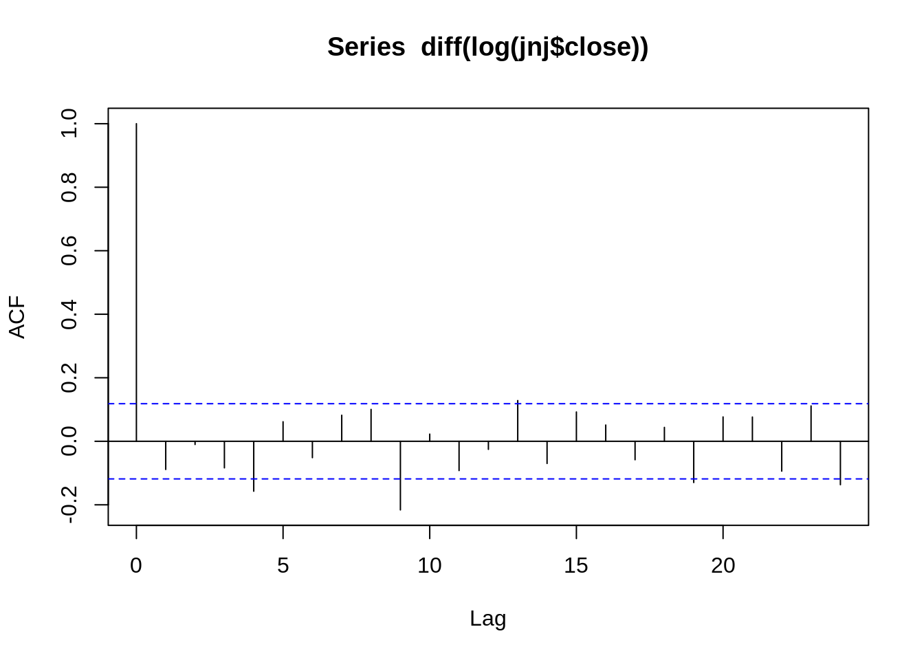
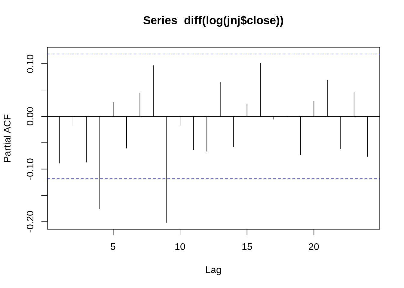
To determine the order of our parameters, we have to look at the difference in lags in both the ACF and PACF graphs. If there is a signficant drop after some lag in the graphs, that suggests the ordered terms we should use for our parameters. For instance, in the ACF graph above, the curve drops significantly after the first lag, so perhaps we should model with one moving average component (MA(1)). While this PACF graph is especially hard to read, let’s say the PACF graph has a significant cut off after 3rd lag, and make it a AR(3) process.
48.4 4. Build the ARIMA Model
Our findings in the ACF/PACF section suggest that model ARIMA(1, 0, 1) might be the best fit. Building an ARIMA model is easy with the forecast package; we just call the function ‘arima’, and specify our parameters.
##
## Call:
## arima(x = diff(log(jnj$close)), order = c(3, 0, 1))
##
## Coefficients:
##          ar1     ar2      ar3      ma1  intercept
##       0.6295  0.0387  -0.0954  -0.7394     0.0056
## s.e.  0.2644  0.0759   0.0775   0.2636     0.0019
##
## sigma^2 estimated as 0.002493:  log likelihood = 432.35,  aic = -852.69
How do we know how well we did? The Akaike information criterion (AIC) score is a good indicator of the ARIMA model accuracy. The lower the AIC score, the better the model performs. Here the model gives us an AIC score of -850.88.
But is that really the best we can do? How would we be able to check this? The answer is through iterated experimentation. We have to randomly experiment with the parameters, until we find the parameters that yield the lowest AIC. Let’s check that assumption by comparing the AIC of this model to other models.
We will use built-in function in forecast called ‘auto.arima’, which will find the best parameters for our model.
A side note: although it can be an easy way out to just use “auto.arima” to find out the best estimated parameters, it is nevertheless a good idea to understand the before steps in order to conduct a prodcutive time series analysis.
##
##  Fitting models using approximations to speed things up...
##
##  ARIMA(2,0,2) with non-zero mean : -864.1353
##  ARIMA(0,0,0) with non-zero mean : -851.583
##  ARIMA(1,0,0) with non-zero mean : -850.7393
##  ARIMA(0,0,1) with non-zero mean : -851.8083
##  ARIMA(0,0,0) with zero mean     : -850.2716
##  ARIMA(1,0,2) with non-zero mean : -851.5652
##  ARIMA(2,0,1) with non-zero mean : -854.3621
##  ARIMA(3,0,2) with non-zero mean : -857.4924
##  ARIMA(2,0,3) with non-zero mean : -847.7652
##  ARIMA(1,0,1) with non-zero mean : -853.6353
##  ARIMA(1,0,3) with non-zero mean : -852.0785
##  ARIMA(3,0,1) with non-zero mean : -856.983
##  ARIMA(3,0,3) with non-zero mean : Inf
##  ARIMA(2,0,2) with zero mean     : -864.44
##  ARIMA(1,0,2) with zero mean     : -846.3745
##  ARIMA(2,0,1) with zero mean     : -851.8578
##  ARIMA(3,0,2) with zero mean     : -851.6499
##  ARIMA(2,0,3) with zero mean     : -862.3785
##  ARIMA(1,0,1) with zero mean     : -848.4336
##  ARIMA(1,0,3) with zero mean     : -846.7636
##  ARIMA(3,0,1) with zero mean     : -853.7823
##  ARIMA(3,0,3) with zero mean     : -855.9012
##
##  Now re-fitting the best model(s) without approximations...
##
##  ARIMA(2,0,2) with zero mean     : Inf
##  ARIMA(2,0,2) with non-zero mean : Inf
##  ARIMA(2,0,3) with zero mean     : Inf
##  ARIMA(3,0,2) with non-zero mean : Inf
##  ARIMA(3,0,1) with non-zero mean : -852.3766
##
##  Best model: ARIMA(3,0,1) with non-zero mean
We get that the best ARIMA model is achieved with parameters p=3, d=0, q=1.
48.5 5. Make Predictions
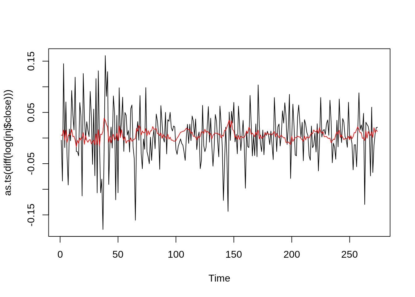
Before we make predictions, let’s see how our model fitted with our training data.
Moving on, we can make a prediction of future stock returns with the forecast.Arima function. We predict the returns on the next 5 months:
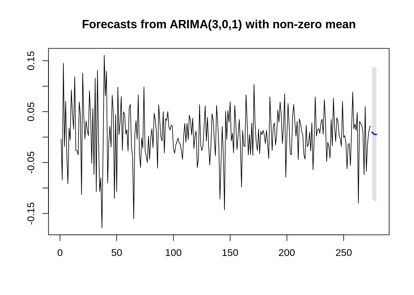
## Time Series:
## Start = 275
## End = 279
## Frequency = 1
## [1] 0.009774685 0.007420760 0.005455234 0.005188938 0.005169821
And we’re done! We can perhaps better determine our model accuracy by using past data and split it into a test and training set, but I wanted to use this as an example of the capabilities of ARIMA in Time Series Modeling.
To conclude, we talked about time series modeling in R. We went over how to stationarize our data, how to determine the order parameters from ACF/PACF, and ultimately how to build our ARIMA model and predict with it. As you can see, time series modeling is a difficult subject, especially in the world of finance, but it can be extremely rewarding as well. Below I have more resources that go more in depth about the various topics I talked about.
48.6 References/Additional Resources
- Chatterjee, Subhasree. “Time Series Analysis Using ARIMA Model In R.” DataScience+, 5 Feb. 2018, https://datascienceplus.com/time-series-analysis-using-arima-model-in-r/
- Dalinina, Ruslana. “Introduction to Forecasting with ARIMA in R.” Oracle Data Science, https://blogs.oracle.com/datascience/introduction-to-forecasting-with-arima-in-r
- Nua, Bob. “Identifying the Numbers of AR or MA Terms in an ARIMA Model.” Identifying the Orders of AR and MA Terms in an ARIMA Model, https://people.duke.edu/~rnau/411arim3.htm.
- Paradkar, Milind. “Forecasting Stock Returns Using ARIMA Model.” R-Bloggers, 9 Mar. 2017, www.r-bloggers.com/forecasting-stock-returns-using-arima-model.
- More info on ARIMA: https://people.duke.edu/~rnau/411arim.htm
- More info on time series stationarity: https://towardsdatascience.com/stationarity-in-time-series-analysis-90c94f27322
- More info on ACF/PACF: https://towardsdatascience.com/significance-of-acf-and-pacf-plots-in-time-series-analysis-2fa11a5d10a8
- More info on AIC: https://www.statisticshowto.datasciencecentral.com/akaikes-information-criterion/