Chapter 26 ggmosaic
Qiang Zhao Mike Yao-Yi Wang
26.1 Overview
This cheat sheet is inspired by the Chapter 15 Chart: Mosaic of the edav.info. Instead of using the mosaic function from the package vcd to plot the mosaic plot, this cheat sheet shows how to achieve the same output through using ggmosaic.
26.2 Introduction
- Mosaic plot is only for categorical data
- Variables to put in
geom_mosaic:- weight: Count/Freq column
- x: product(Y, X2, X1)
- fill: dependent variable Y
- conds: conditional variable
26.3 Order of splits
The mosaic plot follows the hierarchical structure, thus the order of adding variables is very important. Below we will show a step by step splitting by adding one variable at the time. Before going through the example, one must install and call the package ggplot2 and ggmosaic.
library(ggplot2)
library(ggmosaic)

df_bin=data.frame(Age=c('old','old','old','old','young','young','young','young'),
                    Favorite=c(rep('bubble gum',2),rep('coffee',2),rep('bubble gum',2),rep('coffee',2)),
                    Music=c(rep(c('classical','rock'),4)),
                    Freq=c(1,1,3,1,2,5,1,0))
df_unbin = data.frame(Age =c(rep("old",6), rep("young", 8)),
                      Favorite = c(rep("bubble gum", 2),rep("coffee", 4), rep("bubble gum", 7), "coffee"),
                      Music = c("classical", "rock", rep("classical", 3), "rock", rep("classical", 2), rep("rock", 5), "classical"))
26.4 Splitting on One Variable(binned data)
##     Age   Favorite     Music Freq
## 1   old bubble gum classical    1
## 2   old bubble gum      rock    1
## 3   old     coffee classical    3
## 4   old     coffee      rock    1
## 5 young bubble gum classical    2
## 6 young bubble gum      rock    5
## 7 young     coffee classical    1
## 8 young     coffee      rock    0
First, we will show the ggmosaic only split on Age:
Important: The ggmosaic can take binned data by assigning the weight = Freq column of the dataset at its aesthetics, it is not like vcd::mosaic(), which can only take binned data with count column name as Freq.
ggplot(data = df_bin)+
  geom_mosaic(aes(x = product(Age), fill = Age, weight = Freq))+
  labs(x= "Age", title = "Spliting on Age(binned data)")+
  theme(plot.title = element_text(hjust = 0.5))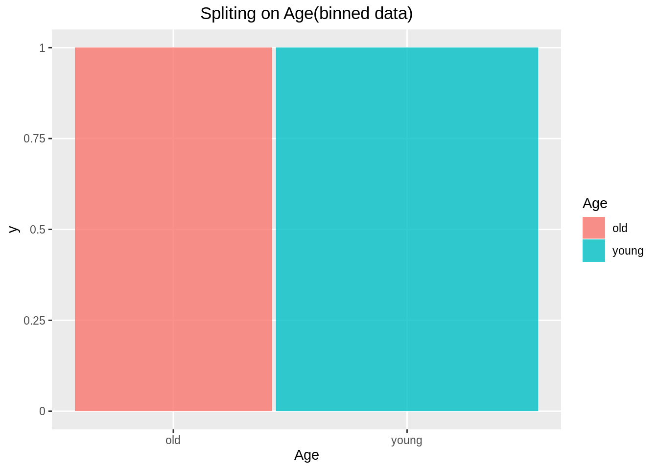
26.5 Splitting on One Variable(unbinned data)
However, for unbinned data, we could just ignore the weight and let it set to default.
The unbinned data:
##      Age   Favorite     Music
## 1    old bubble gum classical
## 2    old bubble gum      rock
## 3    old     coffee classical
## 4    old     coffee classical
## 5    old     coffee classical
## 6    old     coffee      rock
## 7  young bubble gum classical
## 8  young bubble gum classical
## 9  young bubble gum      rock
## 10 young bubble gum      rock
## 11 young bubble gum      rock
## 12 young bubble gum      rock
## 13 young bubble gum      rock
## 14 young coffee classicalggplot(data = df_unbin)+
geom_mosaic(aes(x = product(Age), fill = Age))+
labs(x= "Age", title = "Spliting on Age(unbinned data)")+
theme(plot.title = element_text(hjust = 0.5))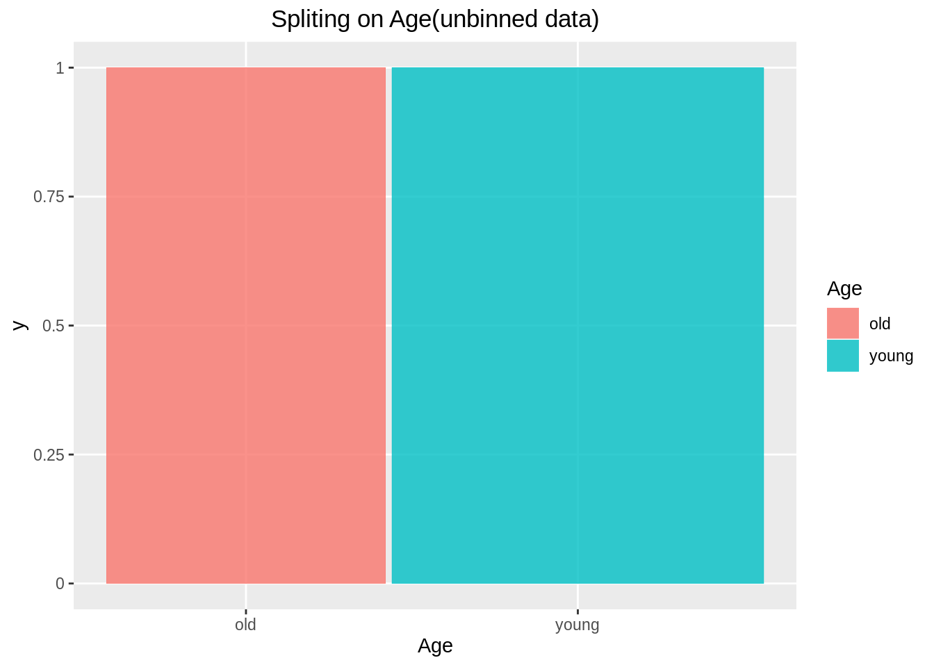
Note: We will use unbinned data for the rest of example
26.6 Splitting on Two Variables
Split on Age, then Music:
ggplot(data = df_unbin)+
  geom_mosaic(aes(x = product(Music, Age), fill = Music))+
  labs(x = "Age", y = "Music", title = "Spliting on Age, then Music")+
  theme(plot.title = element_text(hjust = 0.5))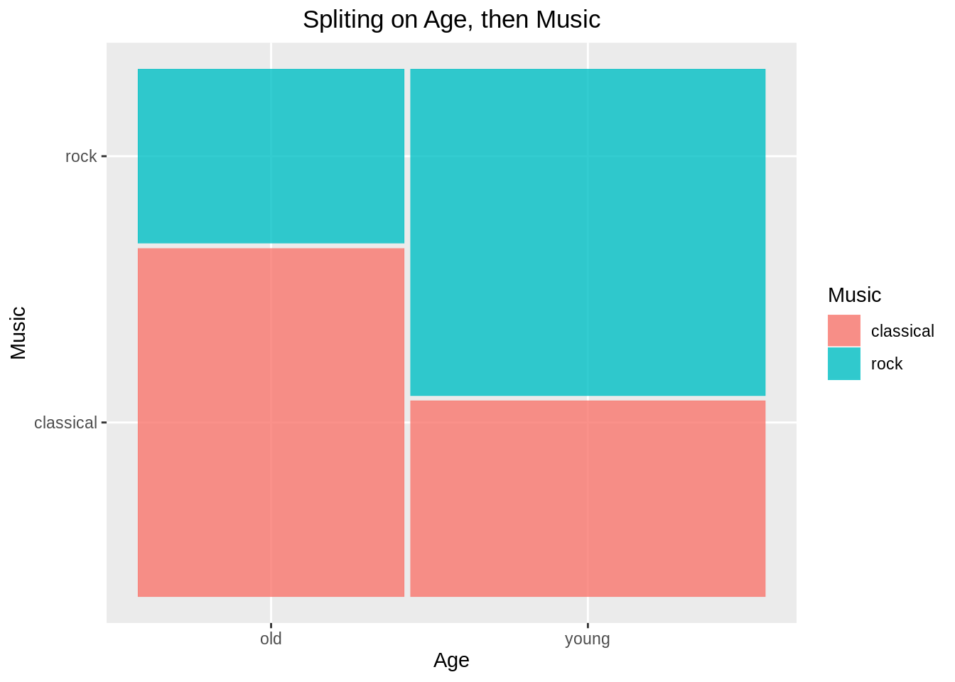
Split on Music, then Age:
ggplot(data = df_unbin)+
  geom_mosaic(aes(x = product(Age, Music), fill = Age))+
  labs(x= "Music", y = "Age",  title = "Spliting on Music, then Age")+
  theme(plot.title = element_text(hjust = 0.5))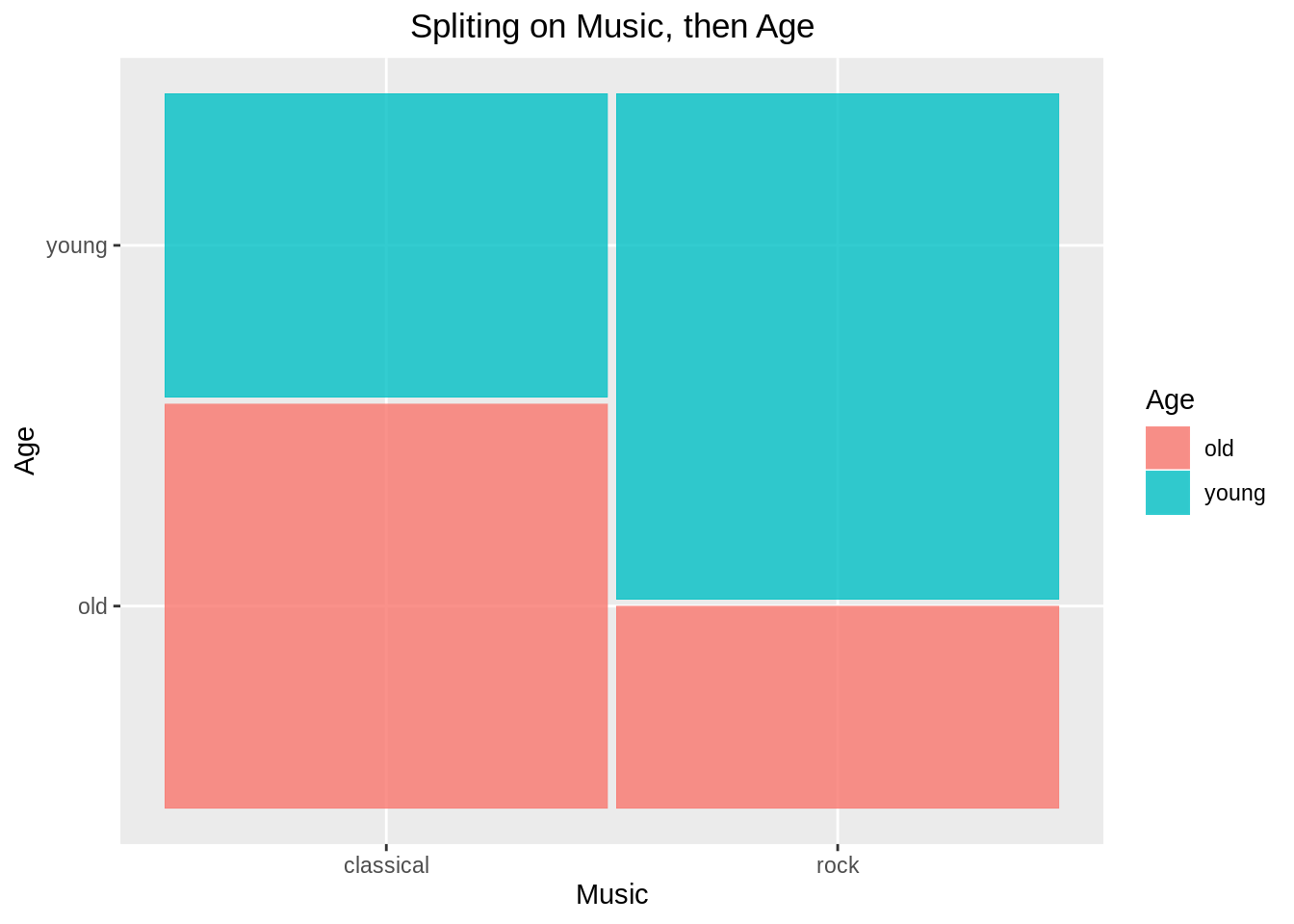
For plotting mosaic plot on Y ~ X, we want to set x = product(Y, X) in aes as we always want to split the dependent variable last. We also need to set fill = Y as we want to color base on dependent variable.
26.7 Splitting on Three Variables
Split on Age, then Music, then Favorite:
ggplot(data = df_unbin)+
  geom_mosaic(aes(x = product(Favorite, Music, Age), fill = Favorite))+
  labs(x = "Favorite:Age", y = "Music", title = "Split on Age, then Music, then Favorite")+
   theme(plot.title = element_text(hjust = 0.5))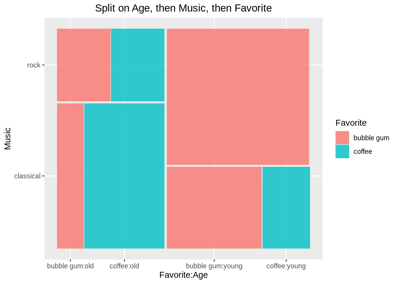
Note that in the above example, by default the order of split and their directions as follows:
Age– vertical splitMusic– horizontal splitFavorite– vertical split
26.8 Adjusting the Direction of Splits
The directions can be adjusted as we want. For example, we want to create a doubledecker plot for the above example following below criteria:
Splitting order:
Age– vertical split (“hspine”)Music– vertical split (“hspine”)Favorite(dependent variable)– horizontal split (“vspine”)
ggplot(data = df_unbin)+
  geom_mosaic(aes(x = product(Favorite, Music, Age), fill = Favorite),
              divider = c("vspine", "hspine", "hspine"))+
  labs(x = "Music:Age", y = "Favorite",
       title = "Doubledecker Plot - Split on Age, then Music, then Favorite")+
  theme(plot.title = element_text(hjust = 0.5))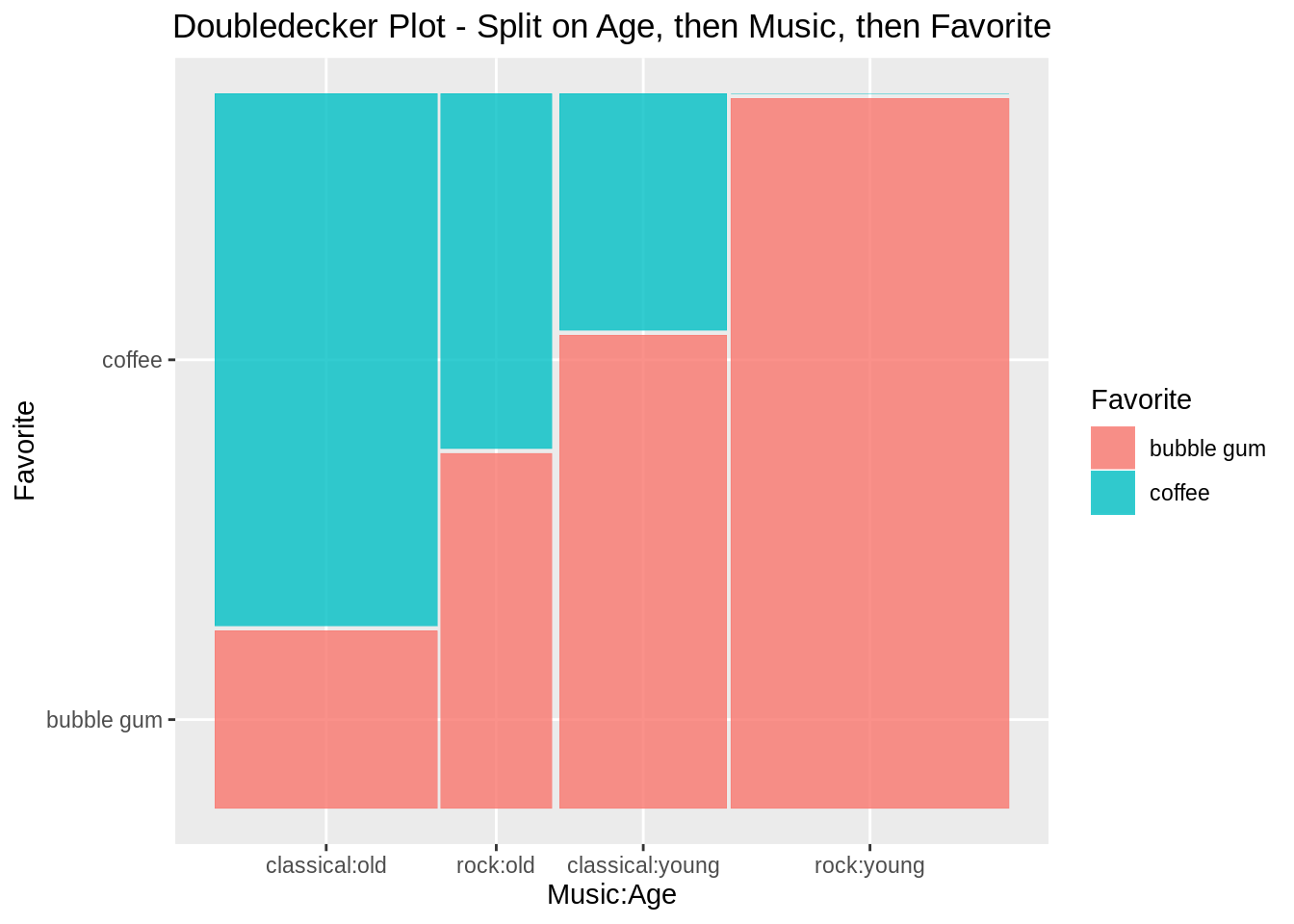
Note that the divider vector is in order of which the variables appear in the product(Favorite, Music, Age), however the order of splits is Age, Music, then Favorite. Also note that in the divider vector, “vspine” = horizontal split and “hspine” = vertical split.
26.9 Alternative approach: Conditional
We can also use conditional property to achieve the same result as the above. In this case, geom_mosaic(aes(x = product(last_split), fill = last_split, conds = product(second_split, first_split)).
ggplot(data = df_unbin)+
  geom_mosaic(aes(x = product(Favorite), fill = Favorite, conds = product(Music, Age)),
              divider = c("vspine", "hspine", "hspine"))+
  labs(x = "Music:Age", y = "Favorite",
       title = "Doubledecker Plot - (Favorite | Music, Age)")+
  theme(plot.title = element_text(hjust = 0.5))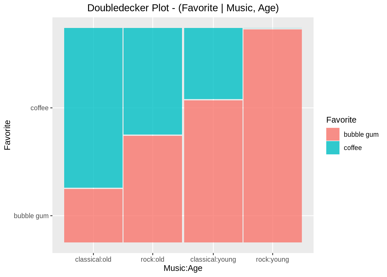
26.10 Alternative approach: Facetting
We can also achieve similar result through facetting.
ggplot(data = df_unbin)+
  geom_mosaic(aes(x = product(Favorite, Music), fill = Favorite))+
  facet_grid(. ~Age)+
  labs(x="Music", y = "favorite", title = "Favorite ~ Music and facet on Age")+
  theme(plot.title = element_text(hjust = 0.5))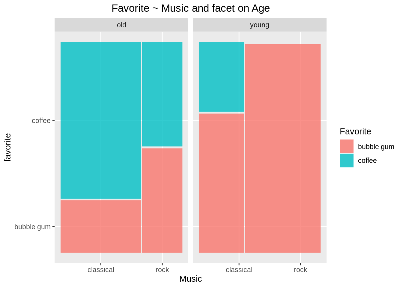
26.11 Comparison with vcd::mosaic
There are often confusions between ggmosaic:geom_mosaic and vcd:mosaic as the syntax for splitting order and splitting direction are quite different for the two. The vcd:mosaic follows the order of mosaic(last_split ~ first_split + second_split) and the direction vector in the order of splits is (first_split, second_split, third_split) with “v” being the vertical split and “h” being the horizontal split. However, ggmosaic:geom_mosaic follow the different pattern, the order of split is product(last_split, second_split, first_split) and the divider (similar to direction in vcd:mosaic) in the order of split is divider = c(last_split, second_split, first_split) with “vspine” being the horizontal split and “hspine” being the vertical split.