Chapter 38 Stamen maps with ggmap
Mrugank Akarte
Here is an example to get started with ggmap using get_stamenmap() to plot the longitude/latitude maps. The data for the following plots is available at https://simplemaps.com/data/us-cities. The get_stamenmap() function reqiures a bounding box, i.e the top, bottom, left and right latitude/longitude of the map you want to plot. For example, the latitude/longitude for US map are as follows:
You can find these values from https://www.openstreetmap.org. The other important parameters of this function are zoom and maptype. Higher the zoom level, the more detailed your plot will be. Beaware that ggmap connects to Stamen Map server to download the map, so if your bounding box is large and zoom level is high, it will have to download a lot of data and may take some time. There are differnt types of plots available via Stamen Map like terrain, watercolor, toner which can be set to maptype parameter according to your preference. You can find about avaiable options in help (?get_stamenmap). For the following examples the maptype is set to ‘toner-lite’.
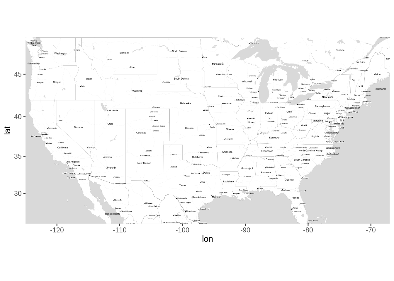
Let’s plot the US map.
Great! We have the US map, now let’s use the US population data to see the spread of counties across nation. Notice that we haven’t included Alaska in the map and hence will be removing the data from Alaska.
library(dplyr)
df <- read.csv(unz('resources/ggmap/data/uscities.zip', 'uscities.csv'))
# Removing data of Alaska from dataset
df <- df %>% filter(state_name != 'Alaska')
# Spread of counties across US using points
ggmap(usmap) +
geom_point(data = df,
mapping = aes(x = lng, y = lat, color = population)) +
ggtitle('Spread of counties across US')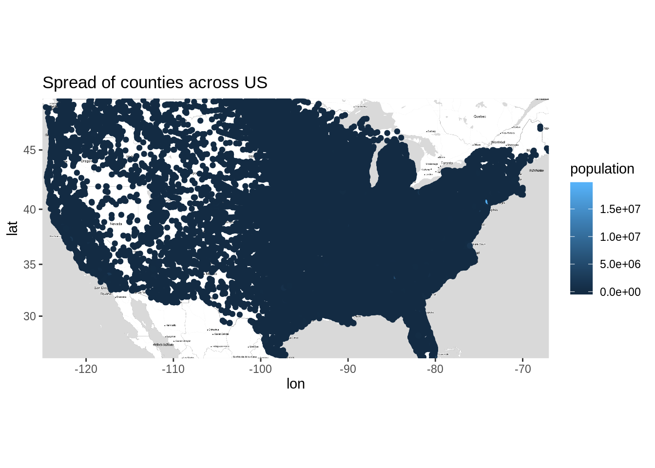
This is not good! Most of the points are overlapping and thus it is not easy to interpret what’s going on here. Let’s try alpha blending and reduce the size of points.
# Spread of counties across US using points
ggmap(usmap) +
  geom_point(data = df,
             mapping = aes(x = lng, y = lat, color = population),
             size = 0.8,
             stroke= 0, alpha = 0.4) +
  ggtitle('Spread of counties across US')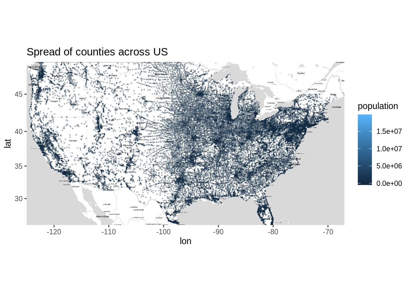
That’s much better! We can now easily identify the areas where number of counties are more. You might have noticed there is no light blue dot visible on the plot. This is because it must be lying somewhere between those dense areas. One such location is New York, you can find this out by zooming the plot. Another reason is that when you use alpha blending, your colors fade and thus it becomes difficult to identify such points.
We can also look at spread of counties using geom_density as follows
# spread of counties across US using Density_2d
ggmap(usmap) +
  geom_density_2d(data = df,
                  mapping = aes(x = lng, y = lat, color = population)) +
  ggtitle('Spread of counties across US')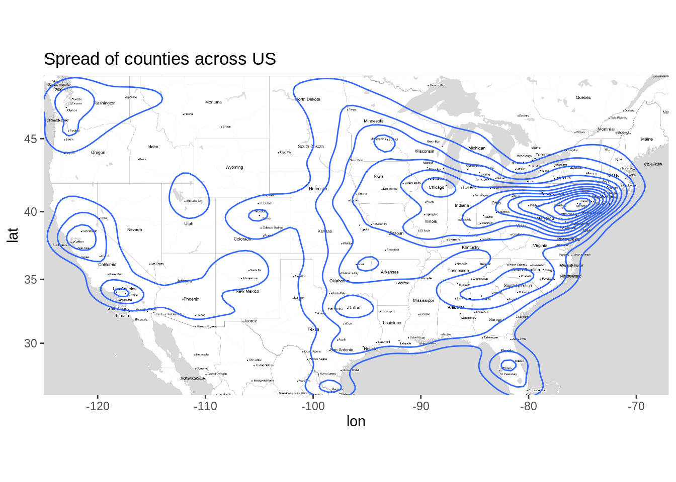
38.1 Mutilayerd plots with ggmaps
We can add multiple layers to the plot as described in earlier chapters. Let’s look at the location of military stations located across US along with population density.
# Location of Military units
df1 <- df %>% filter(military == TRUE)

ggmap(usmap) +
  geom_point(data = df,
             mapping = aes(x = lng, y = lat, color = population, text = city),
             show.legend = F,
             size = 0.8,
             stroke= 0, alpha = 0.4) +
  geom_point(data = df1,
             mapping = aes(x = lng, y = lat , text = city),
             show.legend = F,
             size = 0.9,
             color = 'red') +
  ggtitle('Military stations across US')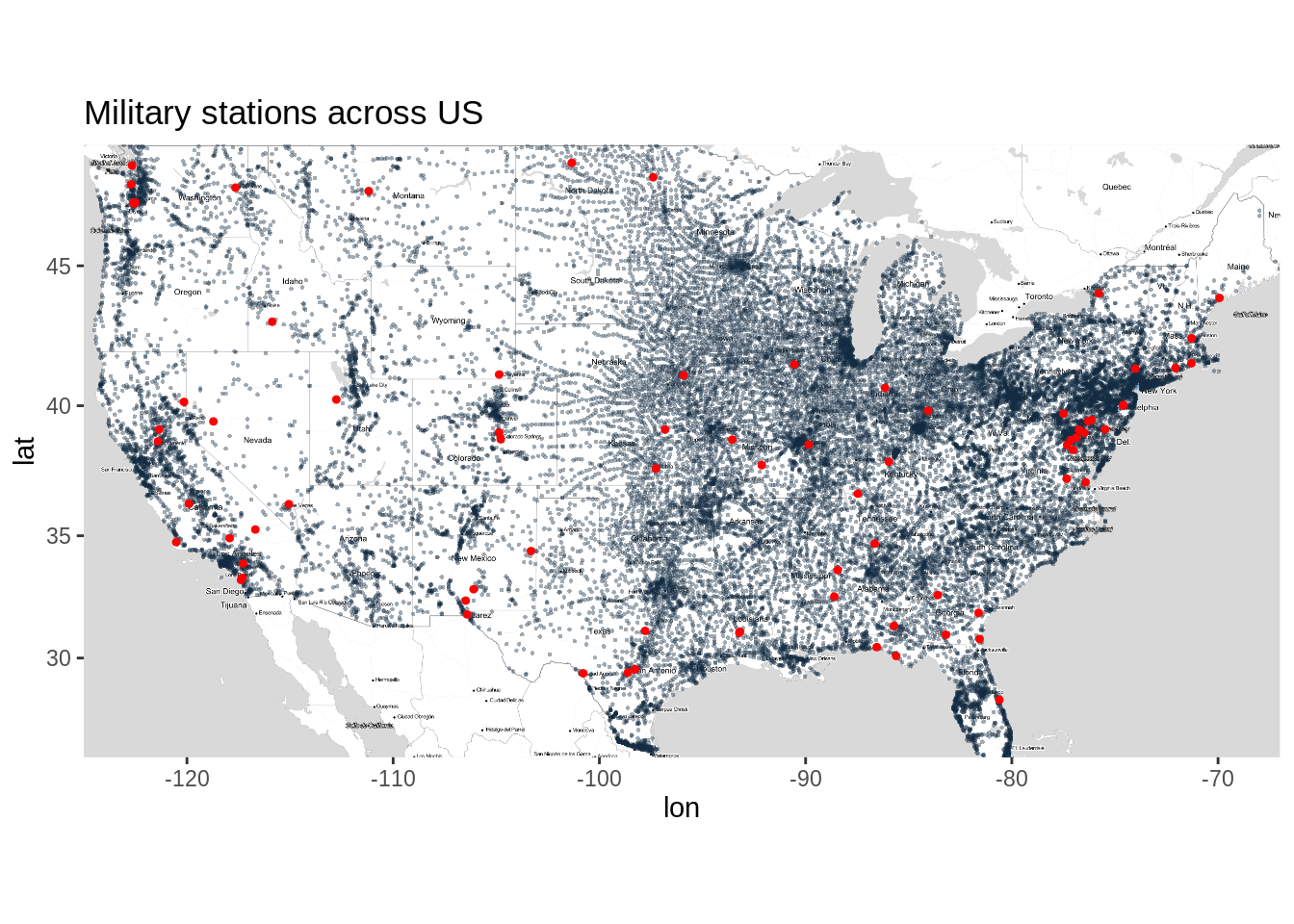
As you can see, there are 3 layers in this plot. First base layer consists of US map, second layer consists of spread of counties across US and the third layer consists of location of military bases. It is not easy to plot such multilayered graphs using other packages.
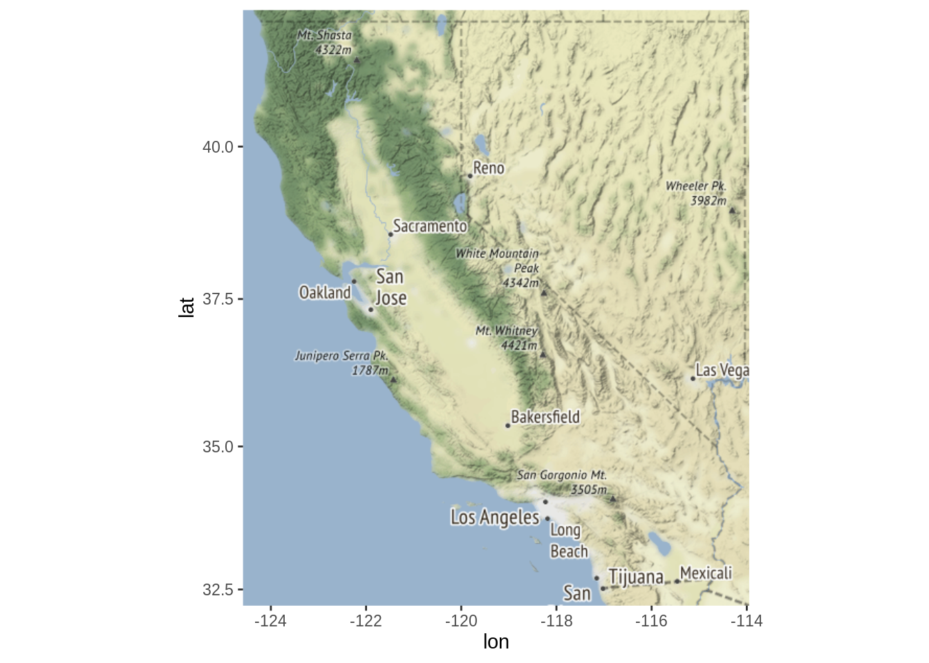
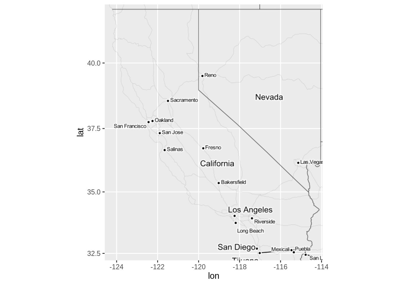
Let’s zoom the map for state of California and see some other map types offered by Stamen Maps.
# California Boundaries
par(mfrow=c(3,1))

CAbox <- c(bottom = 32.213, top = 42.163 , right = -113.95, left = -124.585)
camap1 <- get_stamenmap(bbox = CAbox, zoom = 6, maptype = 'watercolor')
camap2 <- get_stamenmap(bbox = CAbox, zoom = 6, maptype = 'terrain')
camap3 <- get_stamenmap(bbox = CAbox, zoom = 6, maptype = 'toner-hybrid')
ggmap(camap1)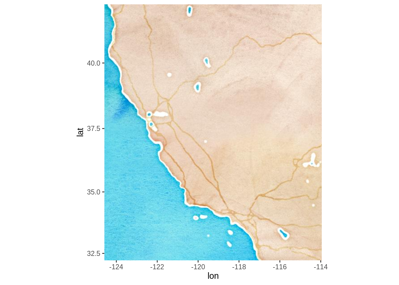
38.2 Getting Deeper
This was just a glimpse of what you can do with ggmaps using the get_stamenmap(). Note that Stamen Maps is not limited to US and can be used to plot any part of the world. If you liked this alternative to Google Maps API, I highly recommend you to check the Stamen Maps website http://maps.stamen.com for more details.