Chapter 18 Visualization in Time Series Analysis
Yihao Li (yl4326)
Note: All the pseudo-documentation introduction will only include parameter I used often, it’s not the full parameter set.
Basic Settings
#In case there's some new package...
#install.packages(c("tidyverse", "stats", "forecast", "dynlm", "lubridate",
#                   "strucchange","sarima"))
library(tidyverse)
library(stats) # a lot of basic operations here
library(forecast) # fantastic package with a ton of shortcut
library(dynlm) # if you need some linear regression on lag of data
library(lubridate) # I didn’t include any function here but necessary for time series
library(strucchange) # parameter stability test
#library(zoo) #used by forecast, will be automatically included
require("PolynomF")
library(sarima) # not for the analysis, just for simulation in showing
18.1 Initiate a Time series object:
stats::ts(data = NA, start = 1, frequency = 1)
where:
data is the data input
start refers to the time of the first observation.
Frequency the number of observations per unit of time.
18.2 Plot the data:
plot(time, value)
Traditional built-in plot,
or,
ggplot2::autoplot(object)
powerful plotting function not only for time series analysis but also for model decomposition object, model fit object, even forecast models.
library(expsmooth) # use a dataset cangas here
ts_data = cangas
autoplot(ts_data) + ylab("Canadaian Gas Production")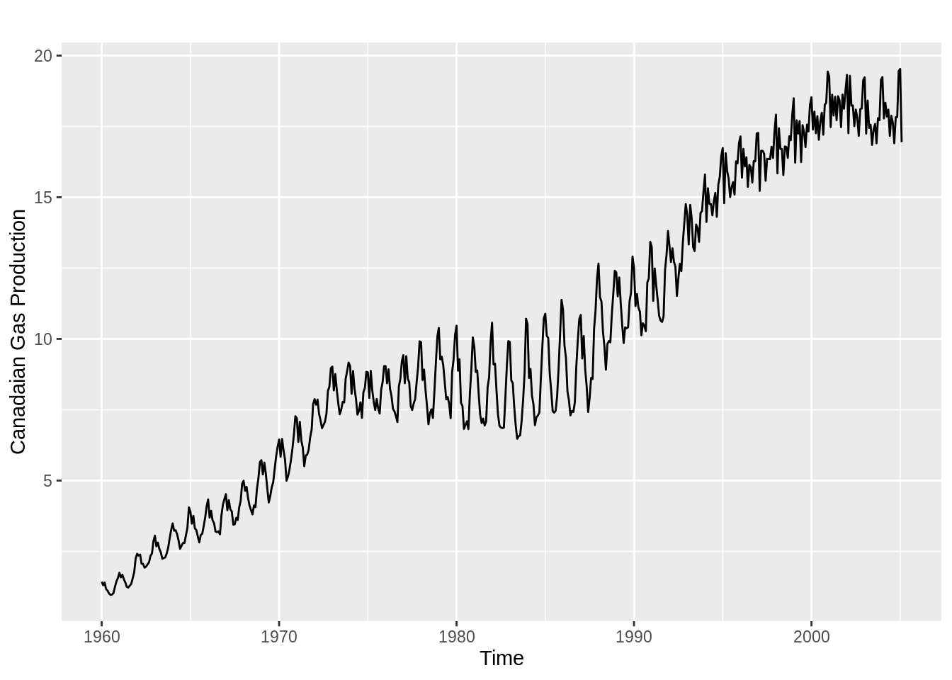
18.3 Transformation of nonstationary:
18.3.1 Stationarity:
Required by most of the time series analysis tools:
1. First Order Weakly Stationary: all R.V.s have the same means.
2. Second Order Weakly Stationary (Covariance Stationary)
a. Necessary for most of the time series analysis.
b. All R.V.s have same variables, same variances.
c. The correlation of time variable only depend on the time difference, i.e. \(\rho(Y_t, Y_{t-k}) = \rho(|k|)\).
18.3.2 Operations
From the plot we have a intuition of its stationarity and we can do following:
1. First Order Weakly Stationary:
Take the first difference \((Y_t – Y_{t-1})\) of the data.
2. second order weakly stationary:
Take the log and then take the first difference(i.e. \((\log(y_T) – \log(y_{T-1}))\)of this transformed series.
3. Growth rate.
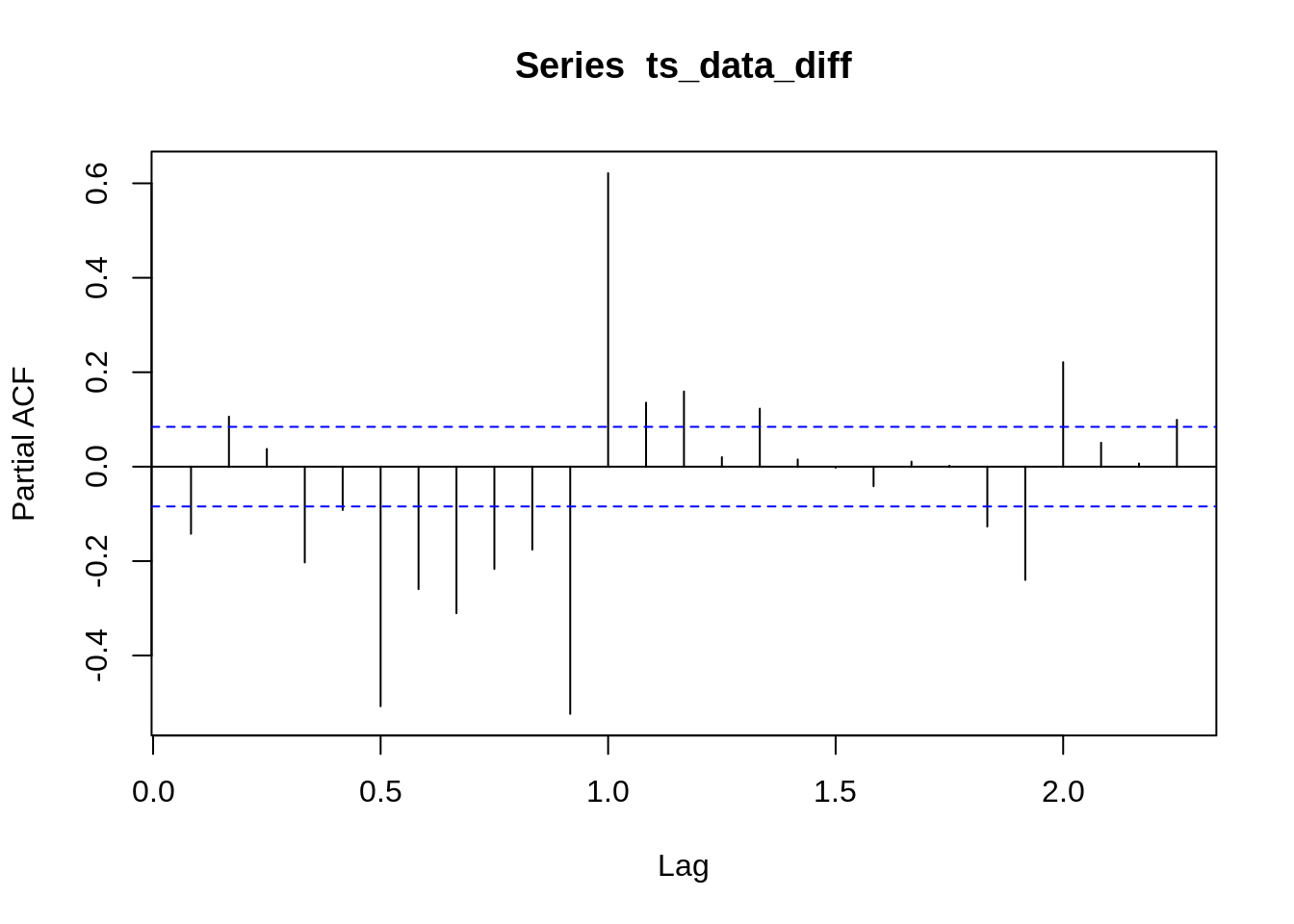
18.4 ACF and PACF for time series
- Autocovariance Function(ACF): \(corr(y_t ,y_{t-k})\)
- Partial Autocorrleation Function(PACF): the autocorrelataion between \(Y_t\) and \(Y_{t+k}\) after removing(conditioning on) all the observation in between.
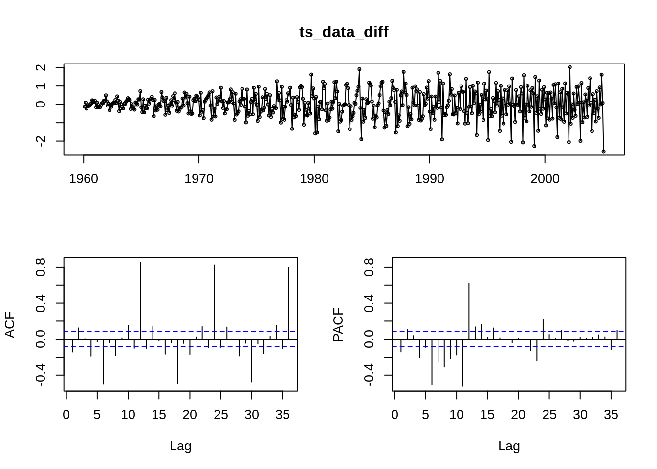
- To save your code line, there’s
forecast::tsdisplay(ts_data)
which plots the ggplot2::autoplot(), stats::acf(), and stats::pacf() together.
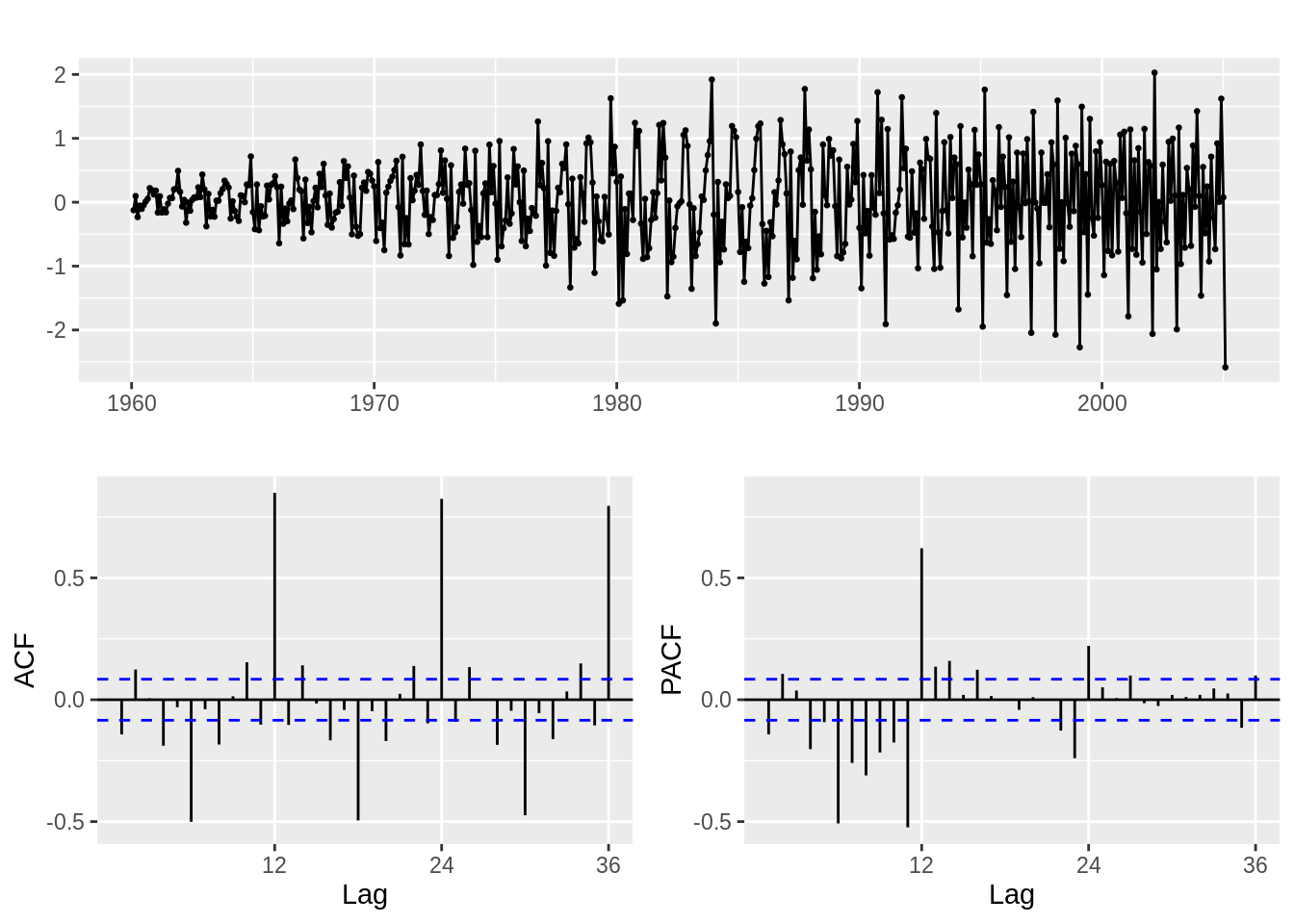
It also have a very friendly
forecast::ggtsdisplay(ts_data)
which returns a ggplot object for you, however, ggtitle() behaves weird in this graph, not to use ggtitle with it. - White Noise:
Time series process with zero mean, constant variance, and no serial correlation.
Most of time use Gaussian y_t ~N(0, \(\sigma\)^2).
For pure white noise, both ACF and PACF should be 0, only k = 0 will have ACF = PACF = 1.

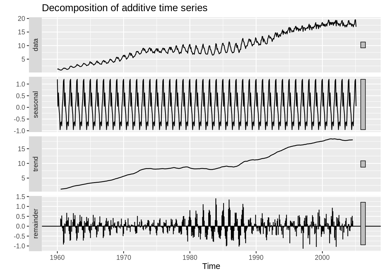
18.5 Full model: Yt = T(Trend) + S(Seasonality) +C(Cycle)
Time is the money my friend, you don’t need to waste time to guess the seasonality pattern.
1. stats::decompose(ts_data, type = c(“additive”, “multiplicative”))
Decompose a time series into seasonal, trend and irregular components using moving average.
Where type stands for additive/multiplicative seasonal cpomponent.
2. stats::stl(ts_data, s.window)
Decompose a time series into seasonal, trend and irregular components using loess.
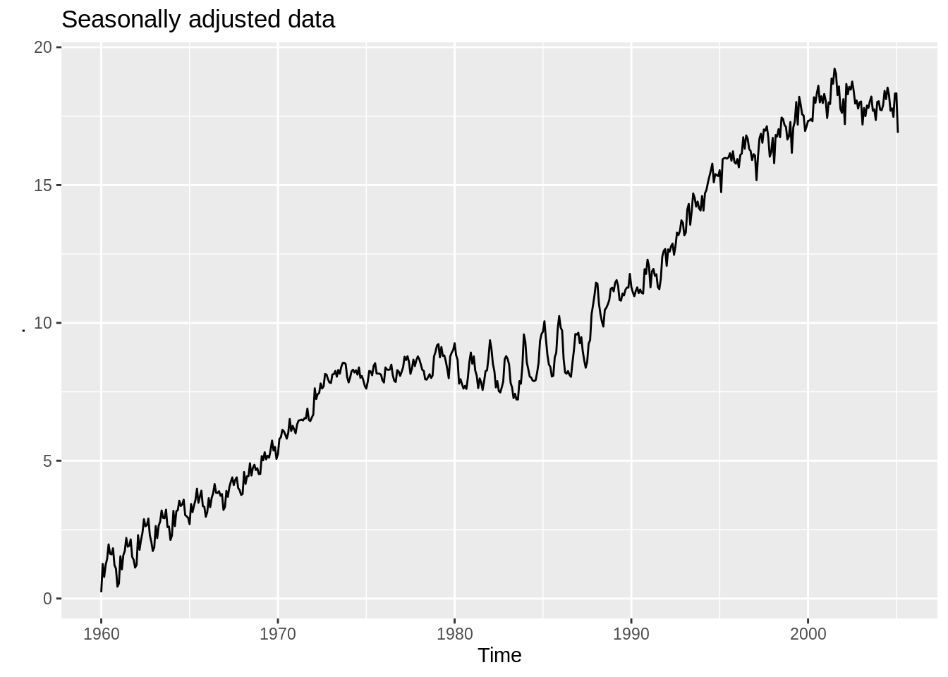
3. forecast::seasadj(object)
Takes in a decompose or stl object. Returns seasonally adjusted data. constructed by removing the seasonal component.
4. You can also find the decomposition data in model.
for decomposed.ts object, it’s in x()(original) seasonal, trend, random(remainder).
for stl object it’s in time.series(seasonal, trend, and remainder).
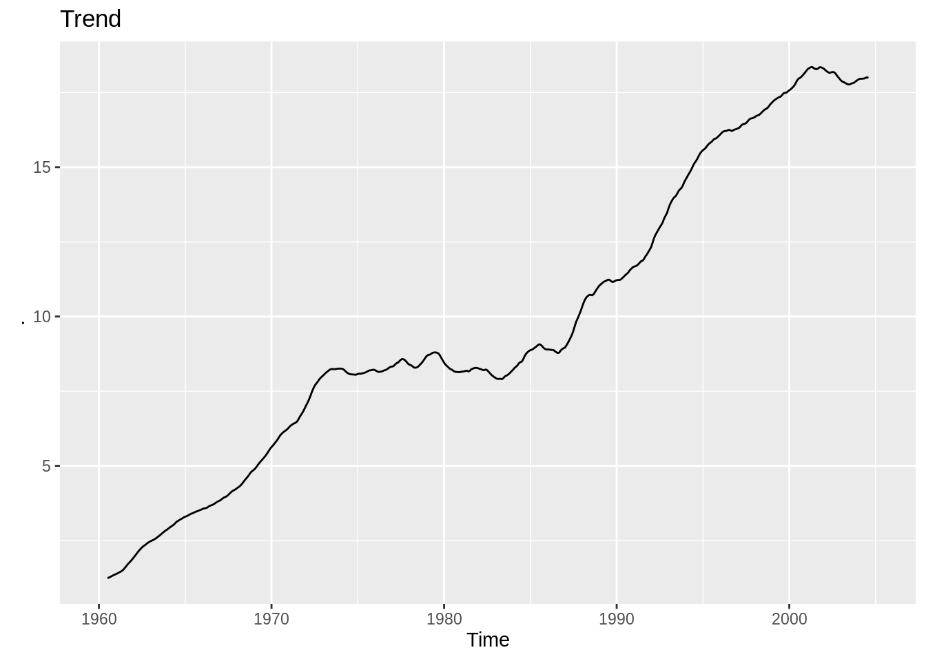
18.5.1 Trend(T): Linear, Quadratic, etc. For normal linear model
stats::lm(formula, data, na.action) For normal linear regression;
dynlm::dynlm(formula, data, na.action) For dynamic linear regression;
na.action is optional but I think it saves life from cleaning data.
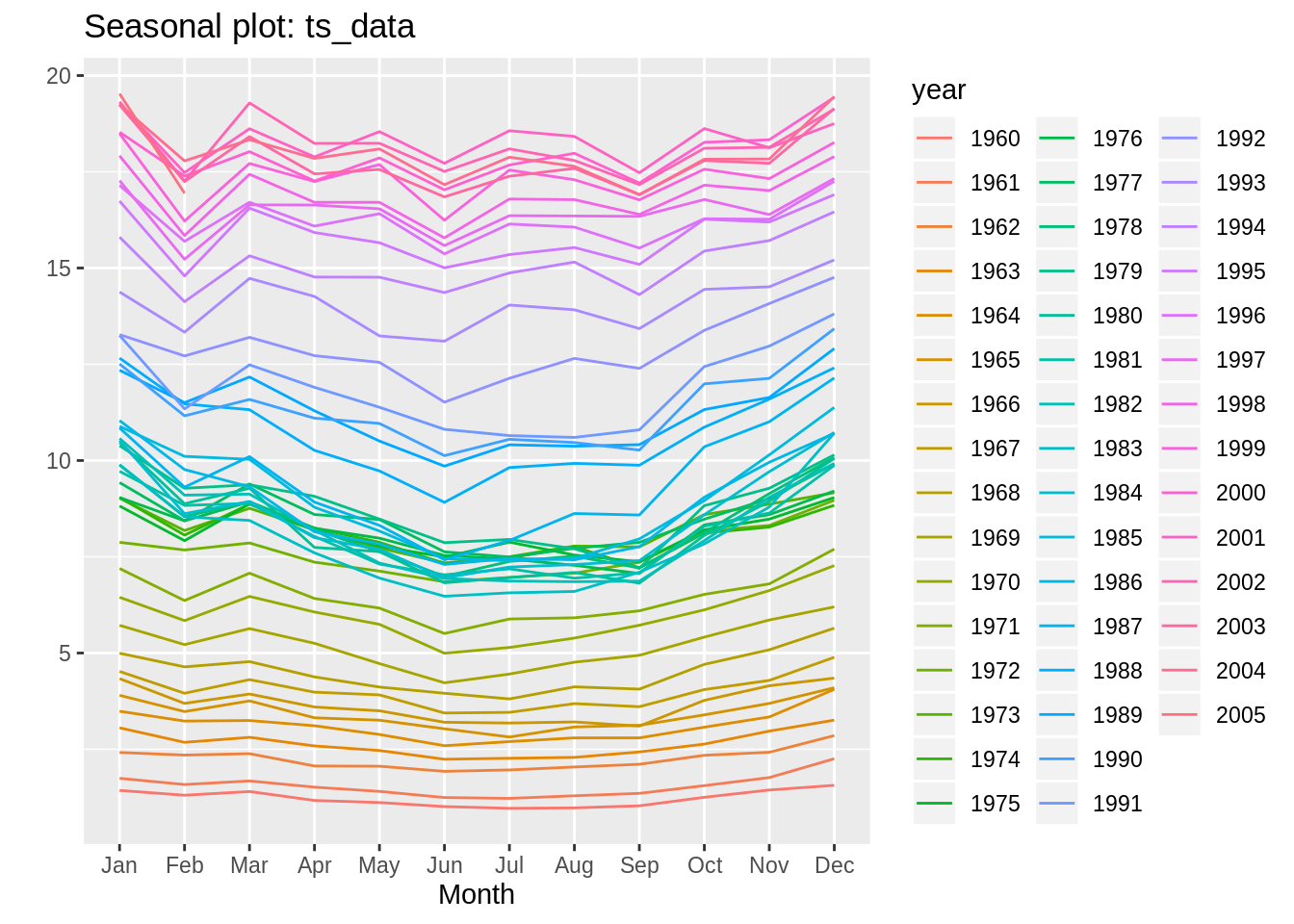
18.5.2 Seasonality(S):
- Direct visualization: decompose and stl.
- one-line beautiful visualization: forecast::seasonplot(ts_data) and it’s ggplot version forecast::ggseasonplot(ts_data).
18.5.3 Cycle(C):
ARIMA family: often used, powerful model in cycle analysis. Notice the model selection is quite subjective except the ARIMA one.
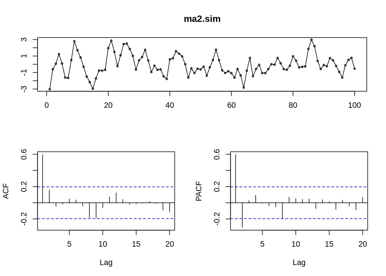
18.5.3.1 1. MA(q) Moving average:
\(Y_t – μ = \sum_1^q \theta_i \epsilon_{t-i}\)
ACF: significant spikes in first q position
PACF: decaying in absolute value
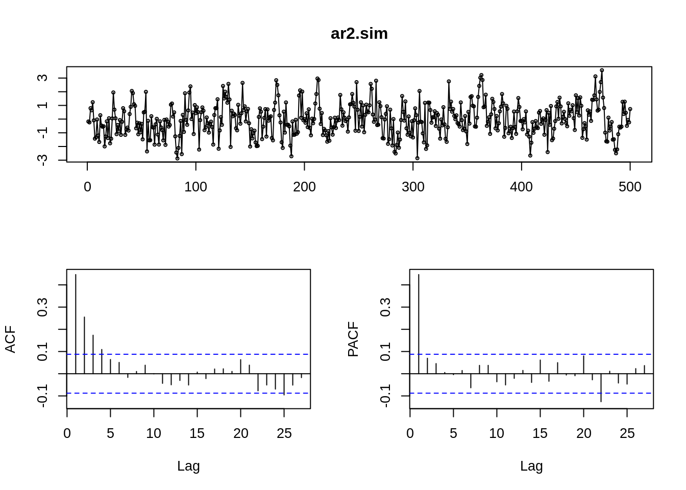
18.5.3.2 2. AR(p) Autoregressive:
\(Y_t = c +\sum_1^p \phi_i Y_{t-i} +\epsilon_t\)
ACF: decaying in absolute value
PACF: significant spikes in first q position.
18.5.3.3 3. Seasonal Model with parameter s:
s stands for the period, e.g. 4 for quarterly data, 12 for monthly data, etc.
18.5.3.3.1 a. Seasonal-MA(q) Model with parameter s:
\(Y_t – μ = \sum_1^q\theta_{is} \epsilon_{t-is} + \epsilon_t\)
ACF: spikes at s, 2s,… , ps
PACF: spikes at ns decaying
s4ma1.sim <- sim_sarima(n=144, model = list(ma=c(rep(0,3),0.8)))
# SMA(1), 4 quarters
tsdisplay(s4ma1.sim)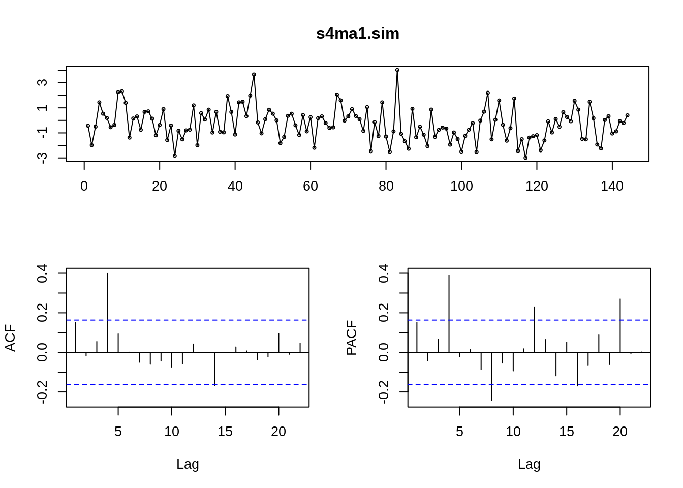
18.5.3.3.2 b. Seasonal-AR(p) Model with parameter s:
\(Y_t = c +\sum_1^p \phi_{is} Y_{t-is} +\epsilon_t\)
ACF: spikes at ns decaying
PACF: spikes at s, 2s,… , ps
s4ar1.sim <- sim_sarima(n=144, model = list(ar=c(rep(0,3),0.8)))
# SAR(1), 4 quarters
tsdisplay(s4ar1.sim)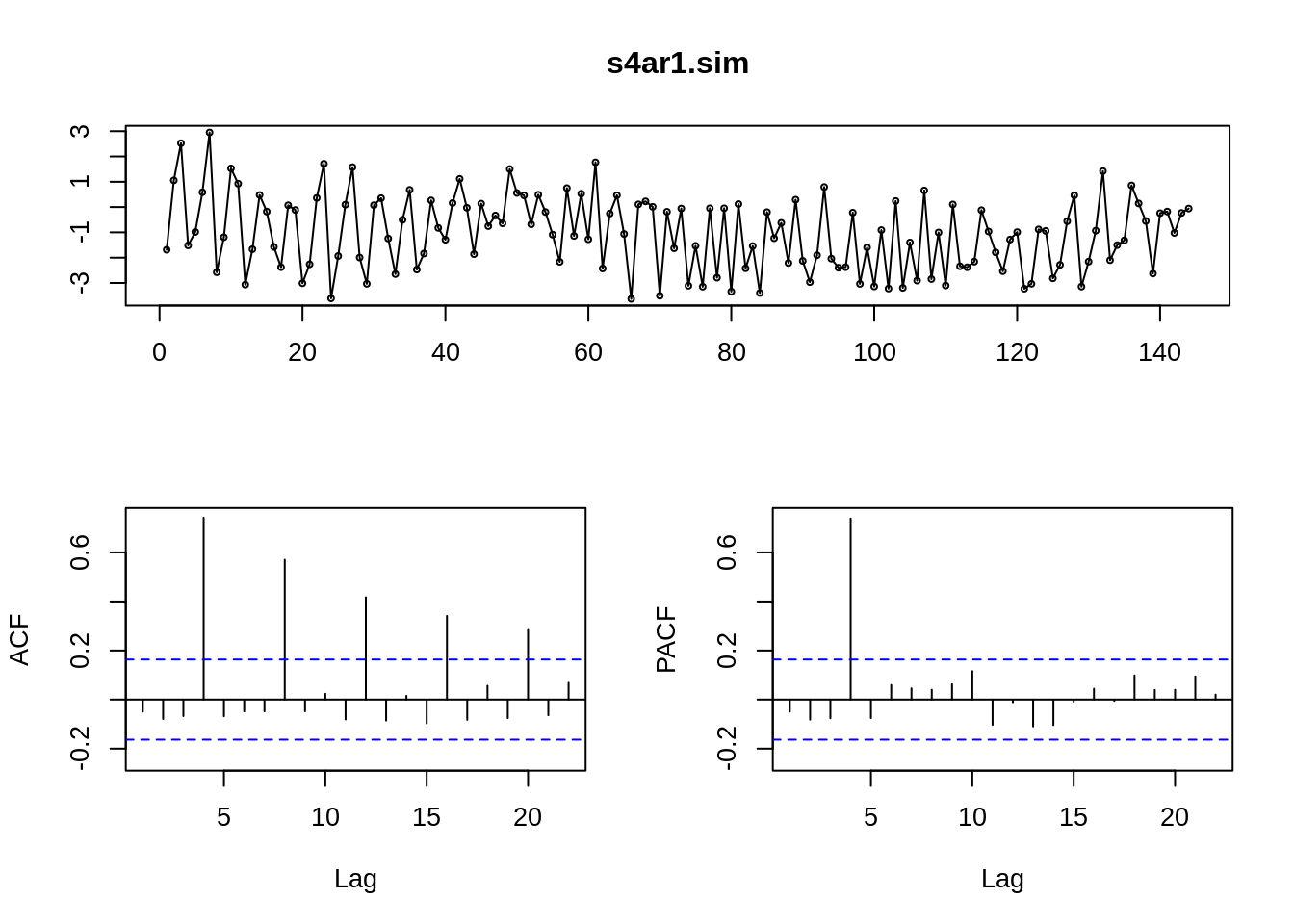
18.5.3.4 4. ARMA(p,q) Autoregressive Moving Average:
- ARMA(p,q) = AR(p) + MA(q), inherited the characters from both AR and MA
- Saves parameters: ARMA(1,1) is performing better than AR(3).
- very subjective in the value selection of p and q…
ar2ma2.sim<-arima.sim(model=list(ar=c(0.9,-0.2),ma=c(-0.7,0.1)),n=100)
#ARMA(2,2)
tsdisplay(ar2ma2.sim)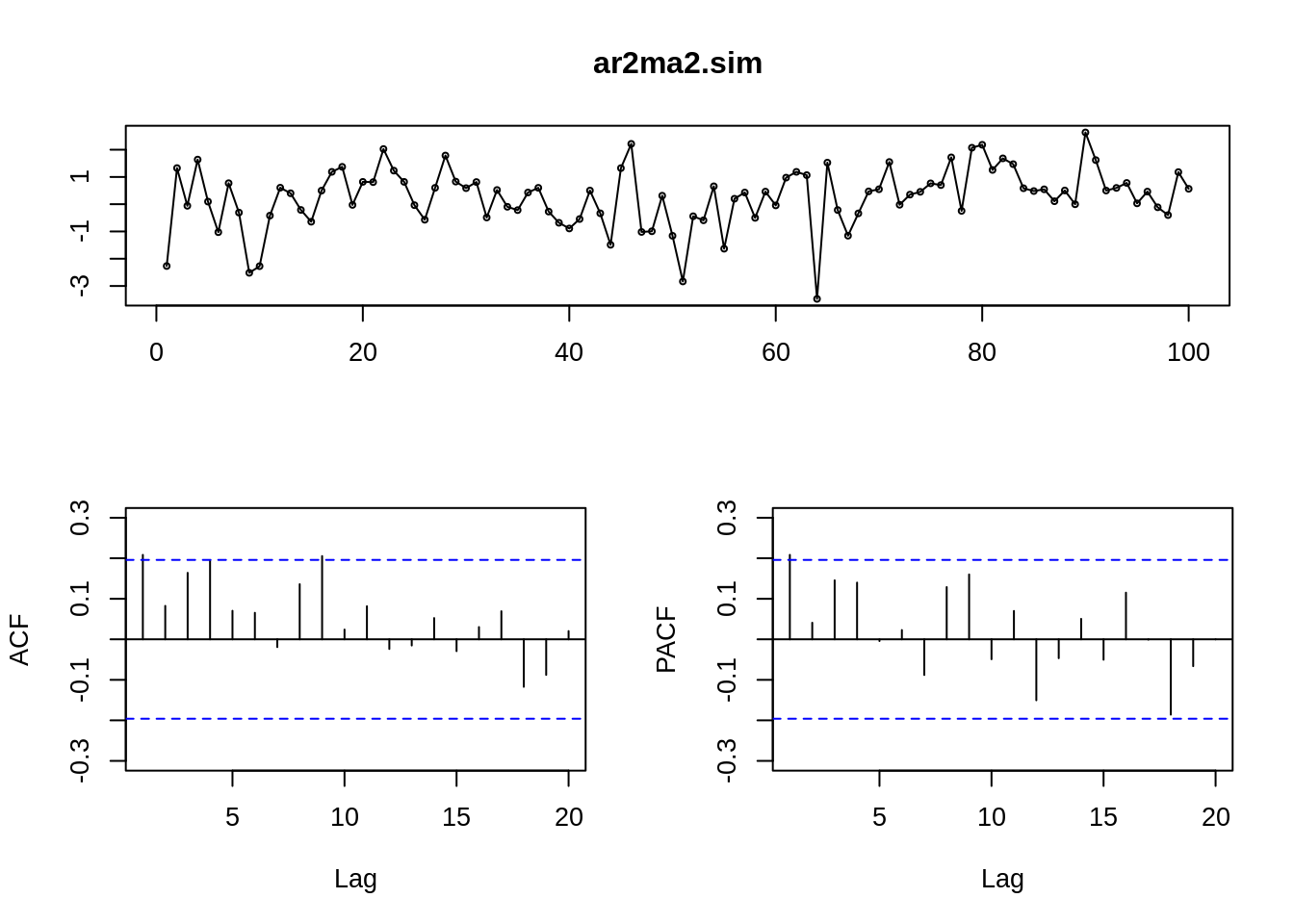
18.5.3.5 5. ARIMA(p,d,q) Autoregressive integrated moving average:
stationary and invertible ARMA(p,q) after differencing d times.
a. Deal with nonstationary series
b. Include d order difference, to remove d or lower order trends.
c. Also deal with stochastic trends
d. Quantitative one-line data choose
forecast::auto.arima(y, ic = c(“aicc”, “aic”, “bic”))
where y is a univariate time series, ic is the criterion.
Returns best ARIMA model with seasonsal ARIMA according to either AIC, AICc or BIC value.
data = read.table("resources/Visualization_in_Time_Series_Analysis/w-gs1yr.txt", header = TRUE)
ts_data = ts(data$rate, start = 1962, deltat = 1/52, freq = 52)
autoplot(ts_data)+ ggtitle("US Weekly Interest Rates (%)")+ ylab("Interest Rate")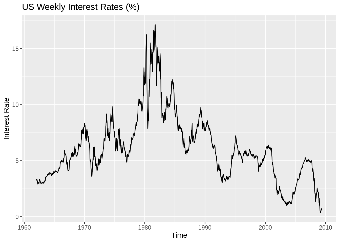
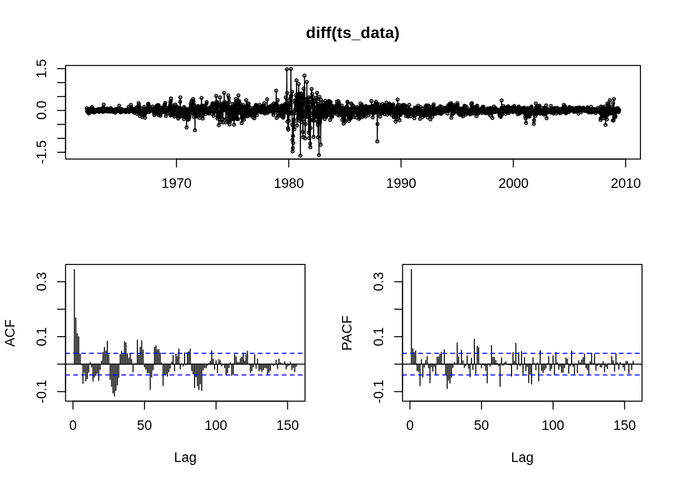
## Series: diff(ts_data)
## ARIMA(1,0,2) with zero mean
##
## Coefficients:
##          ar1      ma1      ma2
##       0.6284  -0.3065  -0.0527
## s.e.  0.0642   0.0675   0.0299
##
## sigma^2 estimated as 0.03143:  log likelihood=768.32
## AIC=-1528.65   AICc=-1528.63   BIC=-1505.41
##
## Training set error measures:
##                         ME      RMSE       MAE MPE MAPE      MASE          ACF1
## Training set -0.0006226569 0.1771898 0.1047296 NaN Inf 0.6423691 -0.0002639336plot(t[-1], diff(ts_data), main = "US Weekly Interest Rates (%) (first difference)", ylab = "Rates",
xlab = "Time", type = "l")
lines(fit$fitted, col = "blue")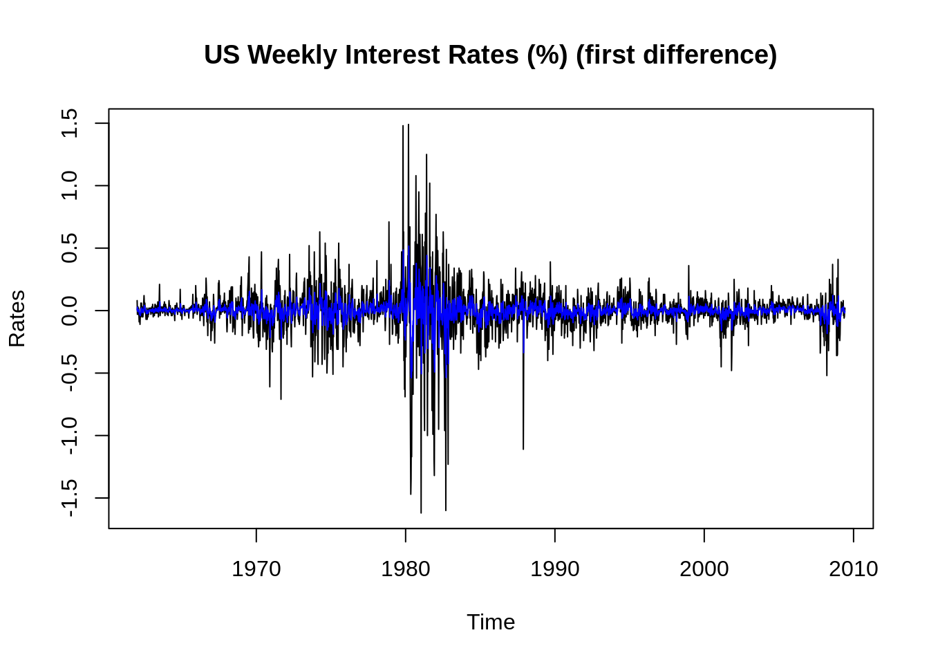
18.5.3.6 Aside:
- AIC(Akaike Information Criterion)
- biased towards overparameterized models
- asymptotically efficient
stats::AIC(fit, k=2)
where:
fit is the a fitted model object,
k is the penalty per parameter to be used; the default k = 2 is the classical AIC.
- BIC/SIC(Bayesian (Schwarz) Information Criterion)
- Consistent
- not asymptotically efficient
stats::BIC(fit)
where fit is the a fitted model object
Both AIC and BIC are the smaller the better.
18.5.4 Summary
18.5.4.1 Steps
The full model includes a trend, seasonal dummies, and cyclical dynamics
For a given visualized data:
a. Extract the trend and seasonality (stl)
b. ACF & PACF, Remove any possible dynamics(tsdisplay, auto.arima)
c. Check if the residuals looks like a white noise
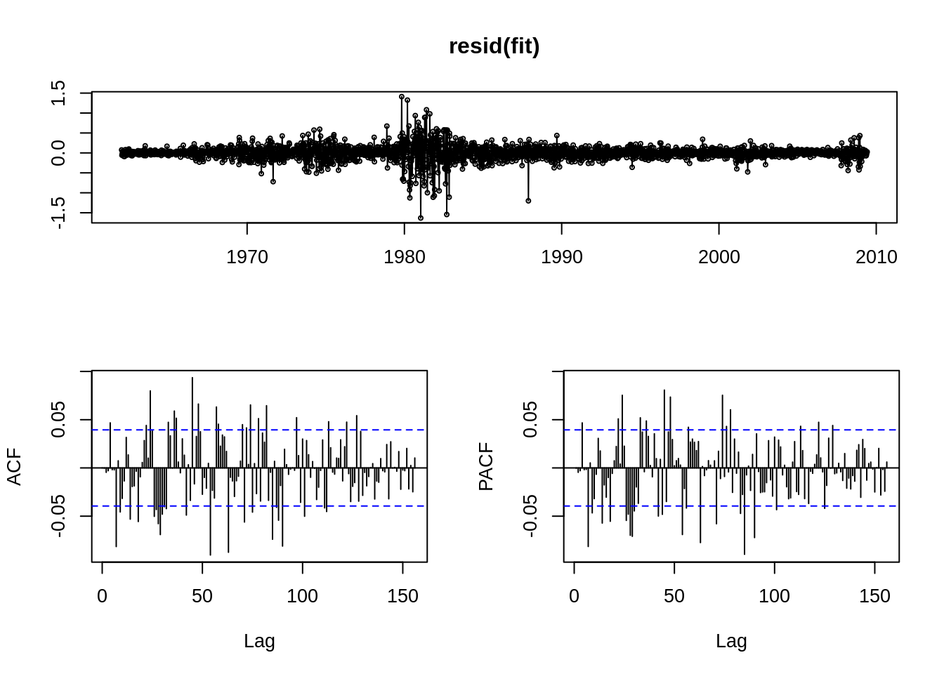
18.5.4.2 Residuals vs White Noise
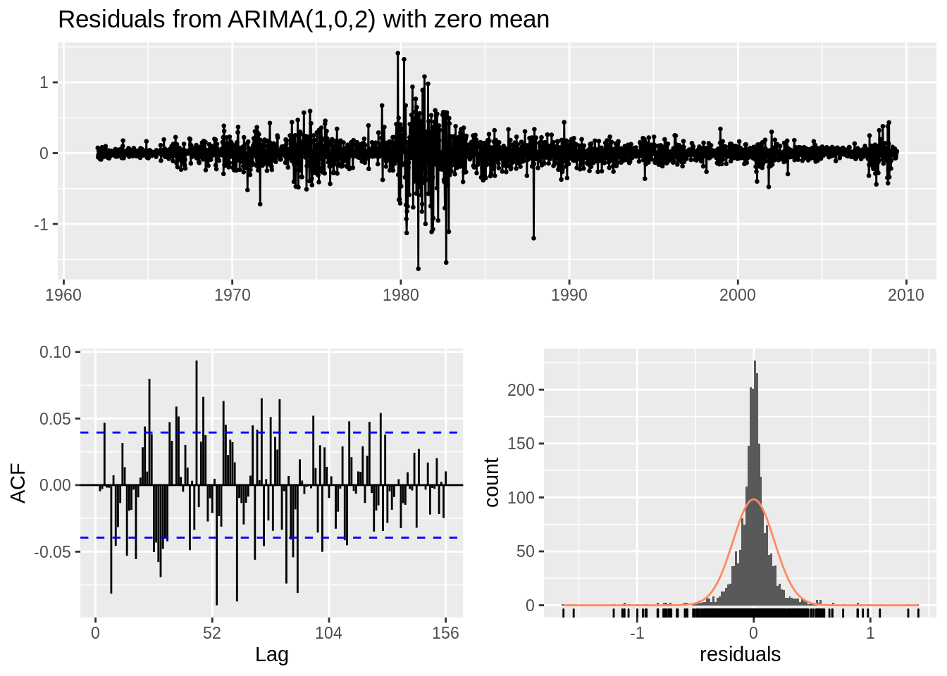
##
##  Ljung-Box test
##
## data:  Residuals from ARIMA(1,0,2) with zero mean
## Q* = 401.53, df = 101, p-value < 2.2e-16
##
## Model df: 3.   Total lags used: 104
Note:
1. Object in resid() can be either a time series model, a forecast object, or a time series (assumed to be residuals).
2. In the new graph, the scale of ACF and PACF is significantly smaller, thus we have removed some of the dynamics.
18.5.4.3 Test Parameter stability
CUSUM(Cumulative Sum of Standardized Recursive Residuals):
Check if the CUSUM leave the confidence interval to capture the dynamics.
Recursive Residuals: strucchange::recresid(x, y, formula)
autoplot(ts(recresid(fit$res ~ t[-1])))+
  ggtitle("The recursive residual of ARIMA(1,0,2)")+
  ylab("recursive residual")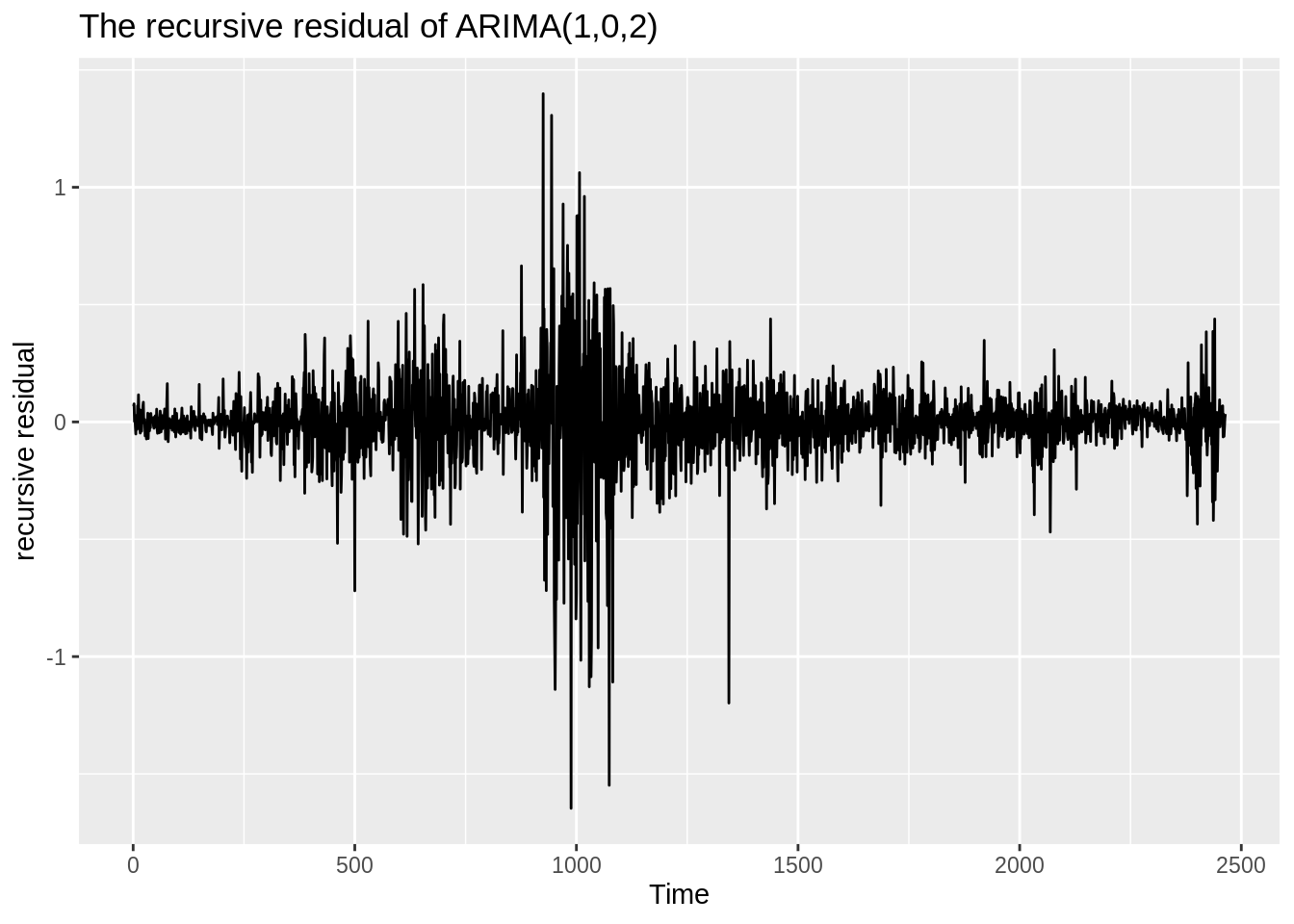
Empirical Fluctuation Processes: efp(x, y, formula, type = “Rec-CUSUM”)
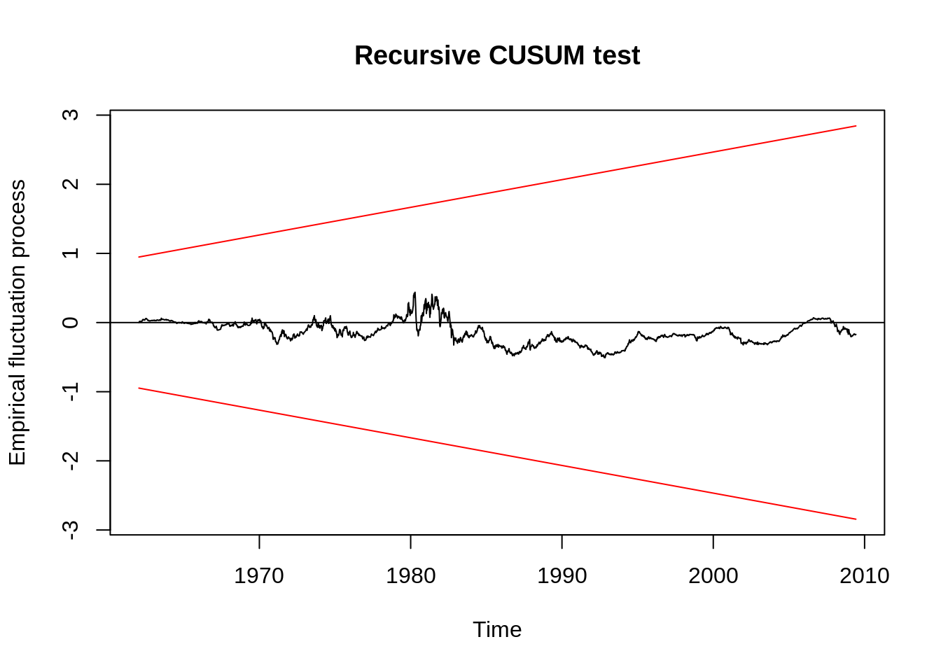
Note:
1. In the recursive residual’s visialization, we find some instability in the middle.
2. Empirical Fluctuation Processes showed the parameter’s stability is acceptable.
18.5.5 Reference:
www.rdocumentation.org
My sincere appreciation to Dr. Randall Rojas (UCLA Econ 144 19’ Spring)’s work. The general model’s idea, both data set: cangas and the tidied “w-gs1yr.txt” is from the Econ 144 class.