25 Animating the plots in R
SeokHyun Kim
25.1 Introduction
gganimate is an interesting extension of the ggplot2 package to create plots with vivid animation in R. In my community contribution project below, I’ll show you how to animate each plots in ggplot2 using strong features in gganimate. You can also customize your graph how it should change with time using this extension.
25.2 Motivation
You should check out the url below. There are amazing plots using gganimate!

Can you imagine these cool fireworks are made using gganimate? Right after I saw that plot in the website, I was truly impressed by what gganimate package can do and decided to share this great visualization package with others!
25.4 Dataset
# I've created dataframe named df which contains speed, strength, win information of each person through year
head(df, 10)
## win strength speed year name
## 1 15 90 22 1995 John
## 2 5 96 19 1996 John
## 3 22 33 20 1997 John
## 4 29 58 24 1998 John
## 5 1 26 25 1999 John
## 6 26 20 24 2000 John
## 7 7 76 17 2001 John
## 8 8 29 15 2002 John
## 9 16 26 24 2003 John
## 10 16 66 19 2004 John
# Below code is used for creating each features
# win <- sample(x=1:30, size=27, replace=T)
# strength  <- sample(x=1:100, size=27, replace=T)
# speed <- sample(x=15:25, size=27, replace=T)
# year <- seq(1995, 2021)
25.5 Understanding transition_states() in gganimate
transition_states() function of gganimate package animates the plot based on a specific variable. (Transition between several distinct states of the data). By specifying variable, which will be the basis, you can obtain GIF image or video representing transition over time or by states.
25.5.1 transition_states() Usage
ggplot(dataframe, aes(x=variable1, y=variable2, ...))+
  geom_graph(...)+
  transition_states(variable3,
                    transition_length=...,
state_length=...)- transition_length : relative length of transition
- state_length : relative length at each state
25.5.2 transition_states() Examples
# Example 1 - barplot
# Before adding transition_states()
ggplot(df, aes(x=name, y=win, fill=name))+
  geom_col(show.legend=FALSE)+
  scale_fill_nord('afternoon_prarie')+
  theme_minimal()+
  facet_wrap(~year)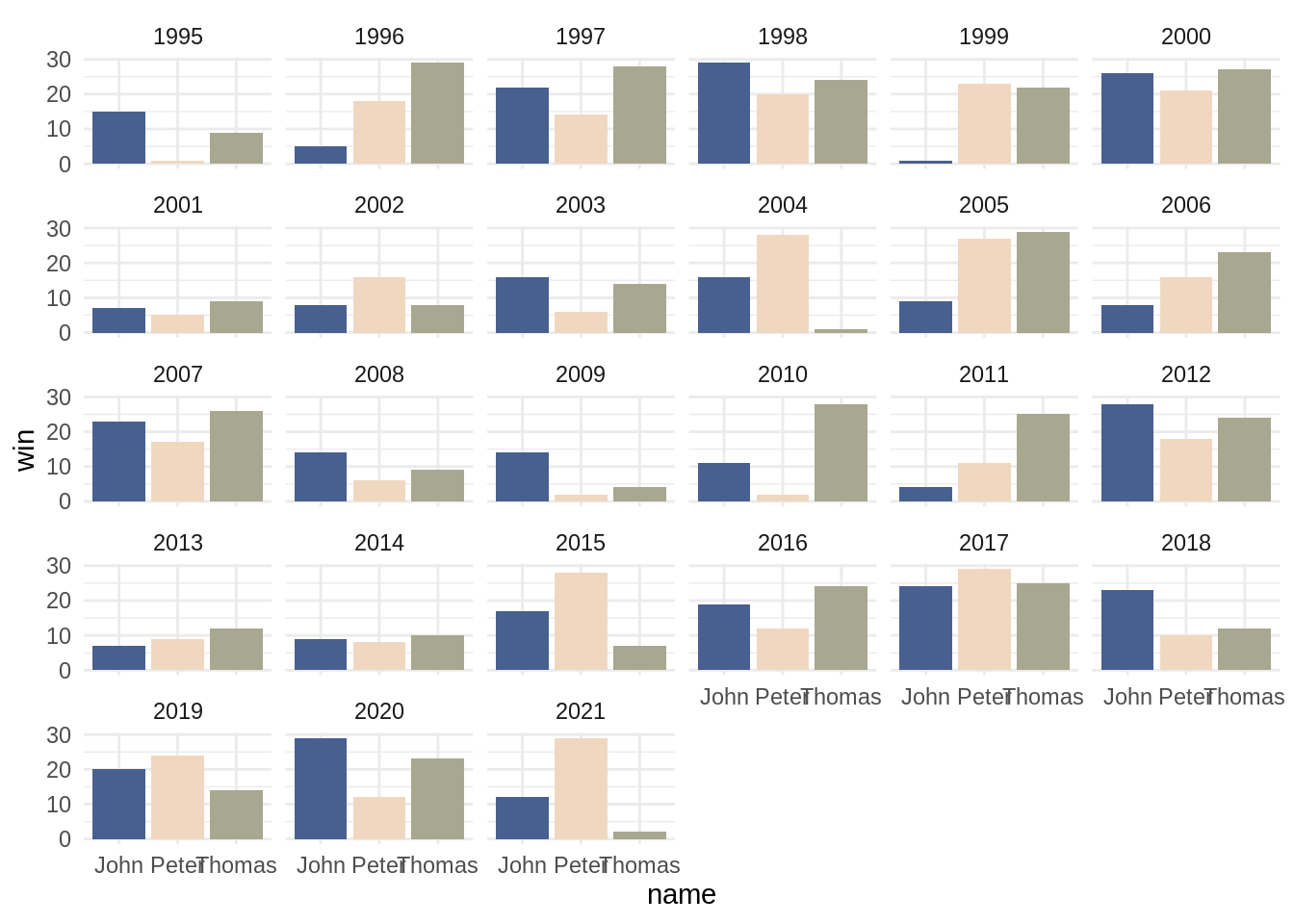
# Example 1 - barplot
# After adding transition_states()
ggplot(df, aes(x=name, y=win, fill=name))+
  geom_col(show.legend=FALSE)+
  scale_fill_nord('afternoon_prarie')+
  theme_minimal()+
  transition_states(year,
                    transition_length=1.5,
                    state_length=0.5)
# Example 2 - scatterplot
# Before adding transition_states()
ggplot(df, aes(x=win, y=strength, color=name))+
  geom_point(size=5, alpha=0.5)+
  scale_color_viridis(option='plasma', discrete=TRUE)+
  theme_minimal()+
  theme(legend.position='bottom')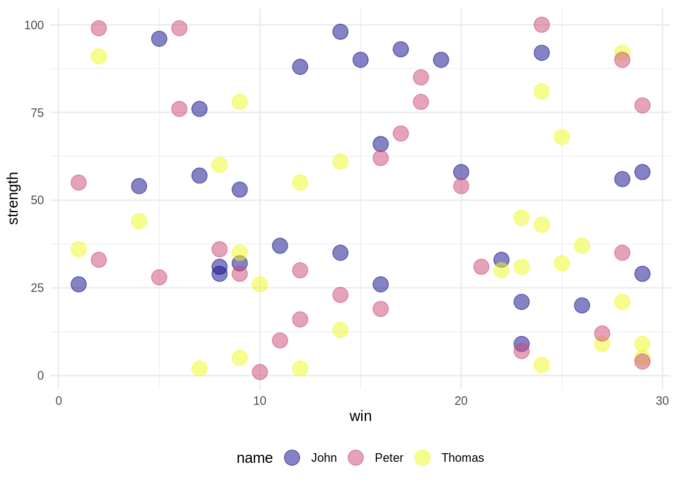
# Example 2 - scatterplot
# After adding transition_states()
ggplot(df, aes(x=win, y=strength, color=name))+
  geom_point(size=5, alpha=0.5)+
  scale_color_viridis(option='plasma', discrete=TRUE)+
  theme_minimal()+
  theme(legend.position='bottom')+
  transition_states(year,
                    transition_length=1.2,
                    state_length=0.2)
25.6 Understanding transition_reveal() in gganimate
transition_reveal() function of gganimate package can create animation so that data is continuously displayed over time when visualizing a given Time Series data into a plot.
25.6.1 transition_reveal() Usage
ggplot(dataframe, aes(x=variable1, y=variable2, group=variable3, ...))+
  geom_line()+
  geom_point()+
  ... +
  transition_reveal(variable1)
25.6.2 transition_reveal() Examples
# Before adding transition_reveal()
ggplot(df, aes(x=year, y=win, group=name, color=name))+
  geom_line()+
  geom_point()+
  scale_color_discrete_sequential('Sunset')+
  theme_minimal()+
  theme(legend.position='bottom')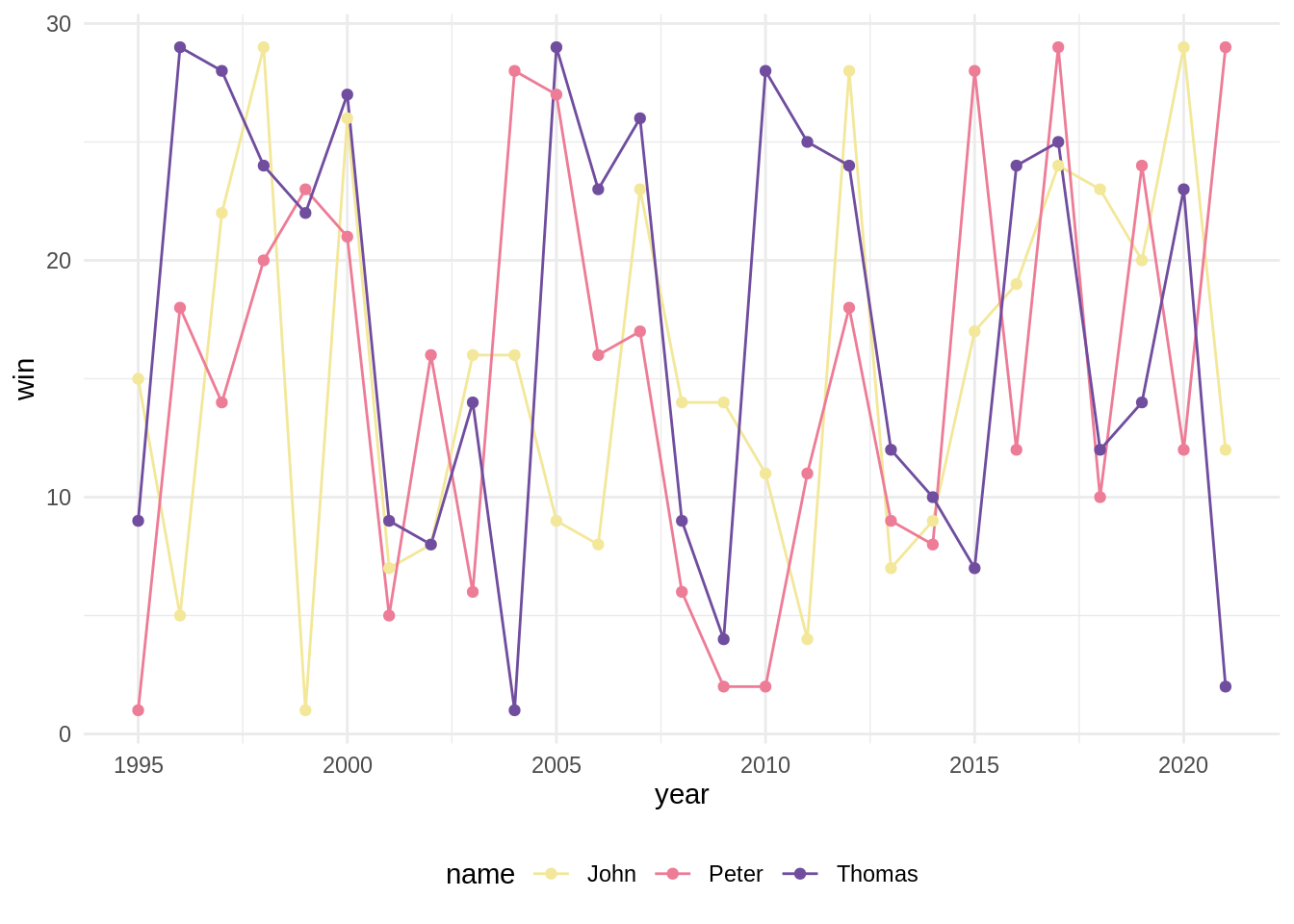
# After adding transition_reveal()
ggplot(df, aes(x=year, y=win, group=name, color=name))+
  geom_line()+
  geom_point()+
  scale_color_discrete_sequential('Sunset')+
  theme_minimal()+
  theme(legend.position='bottom')+
  transition_reveal(year)
25.7 Understanding transition_time() in gganimate
transition_time() function of gganimate package a variant of transition_states(), a tool for visualizing a dataframe indicating the state at a specific point as an animation plot.
25.7.1 transition_time() Usage
ggplot(dataframe, aes(variable1, variable2, ...), ...)+
  geom_point(...)+
  transition_time(variable3)
The length of time to be switched between states is set to be proportional to the interval of actual time between states. Therefore, it is one of the best way to visualize data changes over time.
25.7.2 transition_time() Examples
# Before adding transition_time()
ggplot(df, aes(x=strength, y=win, color=name, size=speed))+
  geom_point(alpha=0.7)+
  scale_color_discrete_sequential('Purple-Yellow', rev=FALSE)+
  scale_y_log10()+
  scale_size(range=c(3,10))+
  theme_minimal()+
  theme(legend.position='bottom')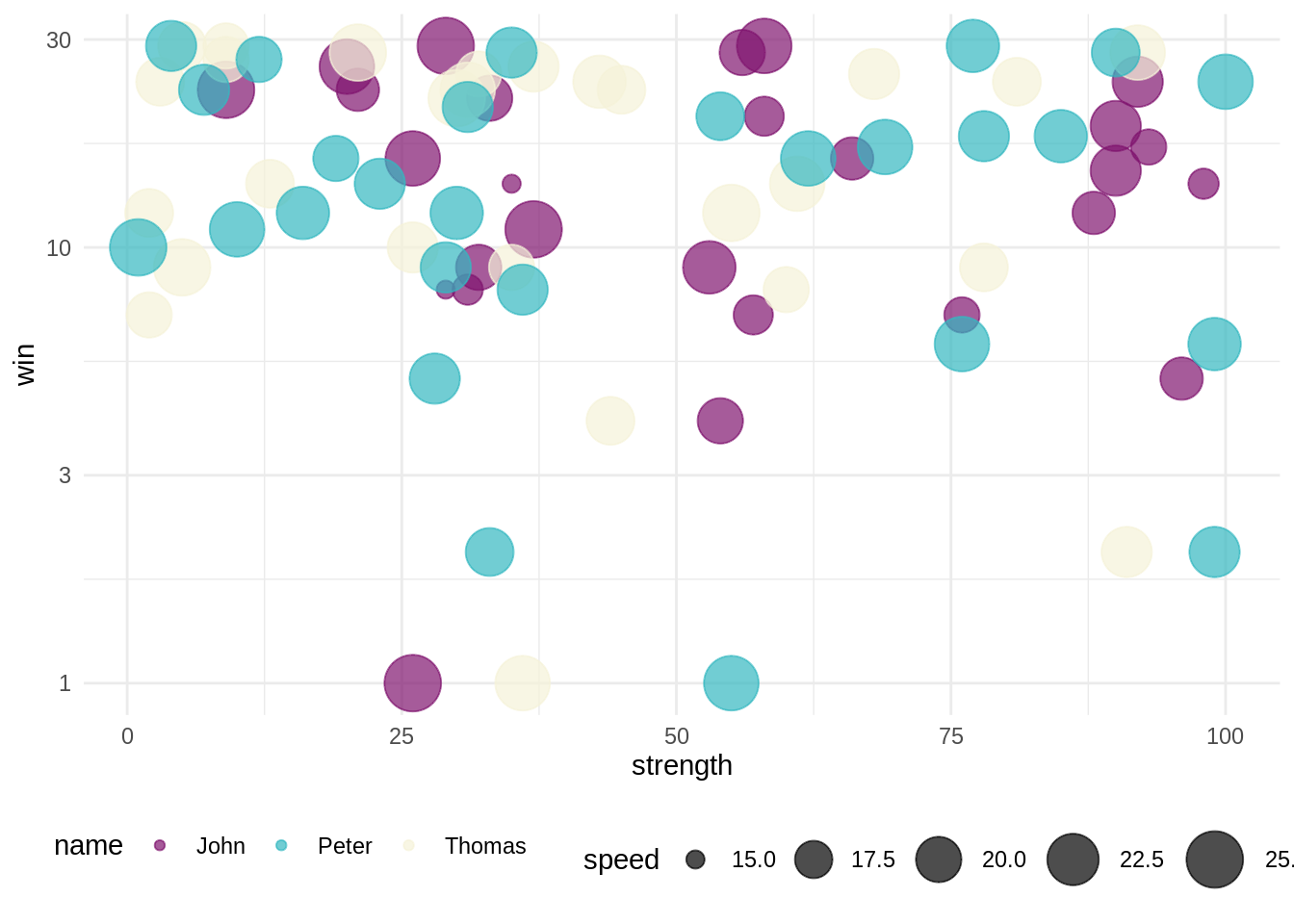
# After adding transition_time()
ggplot(df, aes(x=strength, y=win, color=name, size=speed))+
  geom_point(alpha=0.7)+
  scale_color_discrete_sequential('Purple-Yellow', rev=FALSE)+
  scale_y_log10()+
  scale_size(range=c(3,10))+
  theme_minimal()+
  theme(legend.position='bottom')+
  labs(title='Year: {frame_time}')+
  transition_time(year)
25.8 Understanding shadow_wake() in gganimate
shadow_wake() is a function used with transition_time() or transition_reveal() to shadow the place where changing data has passed. It can be set to gradually reduce the size, color, and transparency of the shadow.
25.8.1 shadow_wake() Usage
ggplot(dataframe, aes(x=variable1, y=variable2, ...))+
  geom_point()+
  ...+
  transition_함수(variable3)+
  shadow_wake(wake_length=0.1, alpha=0)
The length of the shadow can be set at a relative ratio to the total length of the animation, not the frame.
25.8.2 shadow_wake() Examples
# Before adding shadow_wake()
ggplot(df)+
  geom_point(aes(x=strength, y=win, size=speed, color=name))+
  scale_color_viridis(option='viridis', discrete=TRUE)+
  scale_x_log10()+
  scale_size(range=c(1, 3))+
  theme_minimal()+
  theme(legend.position='bottom')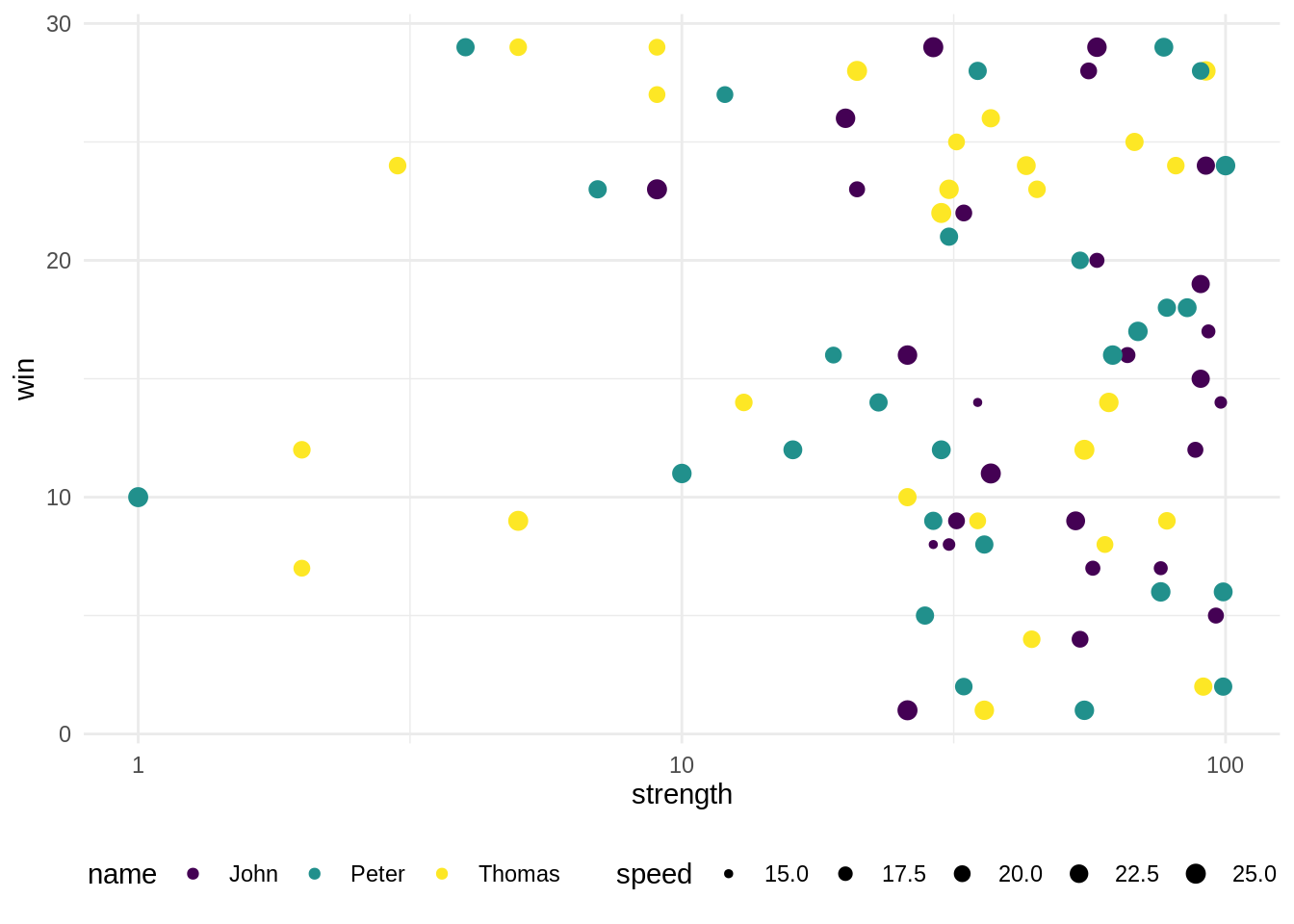
# After adding shadow_wake()
ggplot(df)+
  geom_point(aes(x=strength, y=win, size=speed, color=name))+
  scale_color_viridis(option='viridis', discrete=TRUE)+
  scale_x_log10()+
  scale_size(range=c(1, 3))+
  theme_minimal()+
  theme(legend.position='bottom')+
  transition_reveal(year)+
  shadow_wake(wake_length=0.1,
              alpha=0,
              size=2)
25.9 Conclusion
I covered making animated barplot, scatterplot, timeseries and also shadow using gganimate, but this is just the tip of the iceberg of what this awesome package can do. What I realized during the project is flexibility of the gganimate. Even with the same data, you can generate a lot of different types of plots and also get image or video file through gganimate. For the next time, if I have a chance to work on a project regarding gganimate again, instead of using standardized numeric data, I’ll challenge a completely new way of visualization, as in the example above with fireworks. I encourage you to dive deep into gganimate more!