58 Exploratory data analysis and preprocessing with R for data challenges
Tianhao Wu
58.1 Introduction
Doing a data challenge is usually the first step to get you to a data science job or internship, among which EDA & Data Preprocessing is the most important part because they determine the potential of your model performance and usually give meaningful insights. Most companies have no requirement of building fancy models, instead, they would like to see how you explore and analyze your data, and how you preprocess your data well enough for modeling. In most cases, a good EDA & Preprocessing together with some easy models will get you through the test.
There has been many people sharing solutions for different projects on the internet. However, most of the projects were done in Python, and there is usually a lack of instructions on how to handle a data challenge in general. In this html file, I will share how to perform EDA & Data preprocessing for a typical data challenge with R, using the data of “Iowa House Price Prediction Competition” https://www.kaggle.com/c/iowa-house-price-prediction
58.2 Exploratory Data Analysis & Preprocessing
The first thing is always to have a brief overview of the data with a few questions in mind: How many features do we have? How many of them are numeric? How many of them are categorical? How many categorical features are nominal? These information will affect our strategies in choosing models. For example, if we have a lot of categorical features, then linear models might not work well because they cannot handle categorical features by nature, and encoded categorical features are unlikely to follow a linear relationship.
# read in data and have a brief look
df <- read_csv("resources/r_for_data_challenges/train.csv", show_col_types = FALSE)
num_fea <- df %>% select_if(names(df) != 'SalePrice') %>%
  select_if(is.numeric) %>%
  names()
cat_fea <- df %>% select_if(is.character) %>%
  names()
label <- 'SalePrice'
# explore numeric columns
str(df[,num_fea])
## tibble [1,460 × 37] (S3: tbl_df/tbl/data.frame)
## $ Id : num [1:1460] 1 2 3 4 5 6 7 8 9 10 ...
## $ MSSubClass : num [1:1460] 60 20 60 70 60 50 20 60 50 190 ...
## $ LotFrontage : num [1:1460] 65 80 68 60 84 85 75 NA 51 50 ...
## $ LotArea : num [1:1460] 8450 9600 11250 9550 14260 ...
## $ OverallQual : num [1:1460] 7 6 7 7 8 5 8 7 7 5 ...
## $ OverallCond : num [1:1460] 5 8 5 5 5 5 5 6 5 6 ...
## $ YearBuilt : num [1:1460] 2003 1976 2001 1915 2000 ...
## $ YearRemodAdd : num [1:1460] 2003 1976 2002 1970 2000 ...
## $ MasVnrArea : num [1:1460] 196 0 162 0 350 0 186 240 0 0 ...
## $ BsmtFinSF1 : num [1:1460] 706 978 486 216 655 ...
## $ BsmtFinSF2 : num [1:1460] 0 0 0 0 0 0 0 32 0 0 ...
## $ BsmtUnfSF : num [1:1460] 150 284 434 540 490 64 317 216 952 140 ...
## $ TotalBsmtSF : num [1:1460] 856 1262 920 756 1145 ...
## $ 1stFlrSF : num [1:1460] 856 1262 920 961 1145 ...
## $ 2ndFlrSF : num [1:1460] 854 0 866 756 1053 ...
## $ LowQualFinSF : num [1:1460] 0 0 0 0 0 0 0 0 0 0 ...
## $ GrLivArea : num [1:1460] 1710 1262 1786 1717 2198 ...
## $ BsmtFullBath : num [1:1460] 1 0 1 1 1 1 1 1 0 1 ...
## $ BsmtHalfBath : num [1:1460] 0 1 0 0 0 0 0 0 0 0 ...
## $ FullBath : num [1:1460] 2 2 2 1 2 1 2 2 2 1 ...
## $ HalfBath : num [1:1460] 1 0 1 0 1 1 0 1 0 0 ...
## $ BedroomAbvGr : num [1:1460] 3 3 3 3 4 1 3 3 2 2 ...
## $ KitchenAbvGr : num [1:1460] 1 1 1 1 1 1 1 1 2 2 ...
## $ TotRmsAbvGrd : num [1:1460] 8 6 6 7 9 5 7 7 8 5 ...
## $ Fireplaces : num [1:1460] 0 1 1 1 1 0 1 2 2 2 ...
## $ GarageYrBlt : num [1:1460] 2003 1976 2001 1998 2000 ...
## $ GarageCars : num [1:1460] 2 2 2 3 3 2 2 2 2 1 ...
## $ GarageArea : num [1:1460] 548 460 608 642 836 480 636 484 468 205 ...
## $ WoodDeckSF : num [1:1460] 0 298 0 0 192 40 255 235 90 0 ...
## $ OpenPorchSF : num [1:1460] 61 0 42 35 84 30 57 204 0 4 ...
## $ EnclosedPorch: num [1:1460] 0 0 0 272 0 0 0 228 205 0 ...
## $ 3SsnPorch : num [1:1460] 0 0 0 0 0 320 0 0 0 0 ...
## $ ScreenPorch : num [1:1460] 0 0 0 0 0 0 0 0 0 0 ...
## $ PoolArea : num [1:1460] 0 0 0 0 0 0 0 0 0 0 ...
## $ MiscVal : num [1:1460] 0 0 0 0 0 700 0 350 0 0 ...
## $ MoSold : num [1:1460] 2 5 9 2 12 10 8 11 4 1 ...
## $ YrSold : num [1:1460] 2008 2007 2008 2006 2008 ...
# explore categorical columns
str(df[,cat_fea])
## tibble [1,460 × 43] (S3: tbl_df/tbl/data.frame)
## $ MSZoning : chr [1:1460] "RL" "RL" "RL" "RL" ...
## $ Street : chr [1:1460] "Pave" "Pave" "Pave" "Pave" ...
## $ Alley : chr [1:1460] NA NA NA NA ...
## $ LotShape : chr [1:1460] "Reg" "Reg" "IR1" "IR1" ...
## $ LandContour : chr [1:1460] "Lvl" "Lvl" "Lvl" "Lvl" ...
## $ Utilities : chr [1:1460] "AllPub" "AllPub" "AllPub" "AllPub" ...
## $ LotConfig : chr [1:1460] "Inside" "FR2" "Inside" "Corner" ...
## $ LandSlope : chr [1:1460] "Gtl" "Gtl" "Gtl" "Gtl" ...
## $ Neighborhood : chr [1:1460] "CollgCr" "Veenker" "CollgCr" "Crawfor" ...
## $ Condition1 : chr [1:1460] "Norm" "Feedr" "Norm" "Norm" ...
## $ Condition2 : chr [1:1460] "Norm" "Norm" "Norm" "Norm" ...
## $ BldgType : chr [1:1460] "1Fam" "1Fam" "1Fam" "1Fam" ...
## $ HouseStyle : chr [1:1460] "2Story" "1Story" "2Story" "2Story" ...
## $ RoofStyle : chr [1:1460] "Gable" "Gable" "Gable" "Gable" ...
## $ RoofMatl : chr [1:1460] "CompShg" "CompShg" "CompShg" "CompShg" ...
## $ Exterior1st : chr [1:1460] "VinylSd" "MetalSd" "VinylSd" "Wd Sdng" ...
## $ Exterior2nd : chr [1:1460] "VinylSd" "MetalSd" "VinylSd" "Wd Shng" ...
## $ MasVnrType : chr [1:1460] "BrkFace" "None" "BrkFace" "None" ...
## $ ExterQual : chr [1:1460] "Gd" "TA" "Gd" "TA" ...
## $ ExterCond : chr [1:1460] "TA" "TA" "TA" "TA" ...
## $ Foundation : chr [1:1460] "PConc" "CBlock" "PConc" "BrkTil" ...
## $ BsmtQual : chr [1:1460] "Gd" "Gd" "Gd" "TA" ...
## $ BsmtCond : chr [1:1460] "TA" "TA" "TA" "Gd" ...
## $ BsmtExposure : chr [1:1460] "No" "Gd" "Mn" "No" ...
## $ BsmtFinType1 : chr [1:1460] "GLQ" "ALQ" "GLQ" "ALQ" ...
## $ BsmtFinType2 : chr [1:1460] "Unf" "Unf" "Unf" "Unf" ...
## $ Heating : chr [1:1460] "GasA" "GasA" "GasA" "GasA" ...
## $ HeatingQC : chr [1:1460] "Ex" "Ex" "Ex" "Gd" ...
## $ CentralAir : chr [1:1460] "Y" "Y" "Y" "Y" ...
## $ Electrical : chr [1:1460] "SBrkr" "SBrkr" "SBrkr" "SBrkr" ...
## $ KitchenQual : chr [1:1460] "Gd" "TA" "Gd" "Gd" ...
## $ Functional : chr [1:1460] "Typ" "Typ" "Typ" "Typ" ...
## $ FireplaceQu : chr [1:1460] NA "TA" "TA" "Gd" ...
## $ GarageType : chr [1:1460] "Attchd" "Attchd" "Attchd" "Detchd" ...
## $ GarageFinish : chr [1:1460] "RFn" "RFn" "RFn" "Unf" ...
## $ GarageQual : chr [1:1460] "TA" "TA" "TA" "TA" ...
## $ GarageCond : chr [1:1460] "TA" "TA" "TA" "TA" ...
## $ PavedDrive : chr [1:1460] "Y" "Y" "Y" "Y" ...
## $ PoolQC : chr [1:1460] NA NA NA NA ...
## $ Fence : chr [1:1460] NA NA NA NA ...
## $ MiscFeature : chr [1:1460] NA NA NA NA ...
## $ SaleType : chr [1:1460] "WD" "WD" "WD" "WD" ...
## $ SaleCondition: chr [1:1460] "Normal" "Normal" "Normal" "Abnorml" ...58.2.1 Explore & Handle Numeric Features
Drop useless features like “Id” because they are known to have no influence on our target label. If we don’t drop these columns, they might add noise and lead to overfitting. For example, if IDs were assigned after house prices were sorted, there would be a “strong correlation” between “ID” and “House Price”. As a result, the model would give “ID” a very large weight in predicting house prices, which is not desired at all.
# drop useless features to avoid overfitting & noise
num_fea = num_fea[num_fea != 'Id']
df <- df[,c(num_fea, cat_fea, label)]
Then compute and show the proportions of missing values for each feature.
# show proportions of missing values
missing_col <- colSums(is.na(df[,num_fea]))/dim(df)[1]
missing_col[missing_col > 0] %>% sort(decreasing = TRUE)
## LotFrontage GarageYrBlt MasVnrArea
## 0.177397260 0.055479452 0.005479452- Drop “LotFrontage” because it has too many missing values (proportion > 15%)
- Fill NAs with medians for the rest of numeric features (median is more robust to outliers than mean)
- Always check whether all NAs have been filled
(When using for loop, it is important to use “local({})” to give each iteration a separate local space so that previous results are not overwritten by the most recent one!!)
num_fea <- num_fea[num_fea != 'LotFrontage']
df <- df[,c(num_fea, cat_fea, label)]
for (i in c('GarageYrBlt','MasVnrArea')) {
  df[is.na(df[i]), i] <- local({
    i <- i
    median(unlist(df[i]), na.rm=TRUE)
  })
}
missing_col <- colSums(is.na(df[,num_fea]))/dim(df)[1]
missing_col[missing_col > 0] %>% sort(decreasing = TRUE)
## named numeric(0)Use multiple scatter plots to explore the relationships between some important features and the label. Here I choose features based on their correlation coefficients with the label. The reason we want to visualize these relationships are as follows:
- Are there any outliers or unexpected patterns?
- Are there any features we assume to be highly correlated with the label but not displayed here (because of low correlation coefficients (<0.4))?
- After we train our models, we should come back and check whether the feature importance returned by models are aligned with our observation here. If there are any interesting differences, we should explore the reasons behind.
corr <- cor(df[,append(num_fea, label)])[,label]
corr <- corr[order(abs(corr), decreasing = TRUE)]
imp_num_fea <- names(corr[abs(corr)>0.4]) # only take the features with absolute value of coeff > 0.4
imp_num_fea <- imp_num_fea[imp_num_fea != label]

p <- list()
for (i in 1:length(imp_num_fea)) {
  p[[i]] <- local({
    i <- i
    ggplot() +
    geom_point(aes(x=unlist(df[,imp_num_fea[i]]), y=unlist(df[label]))) +
    xlab(imp_num_fea[i]) +
    ylab("House Prices")
  })
}
grid.arrange(grobs = p, ncol = 3)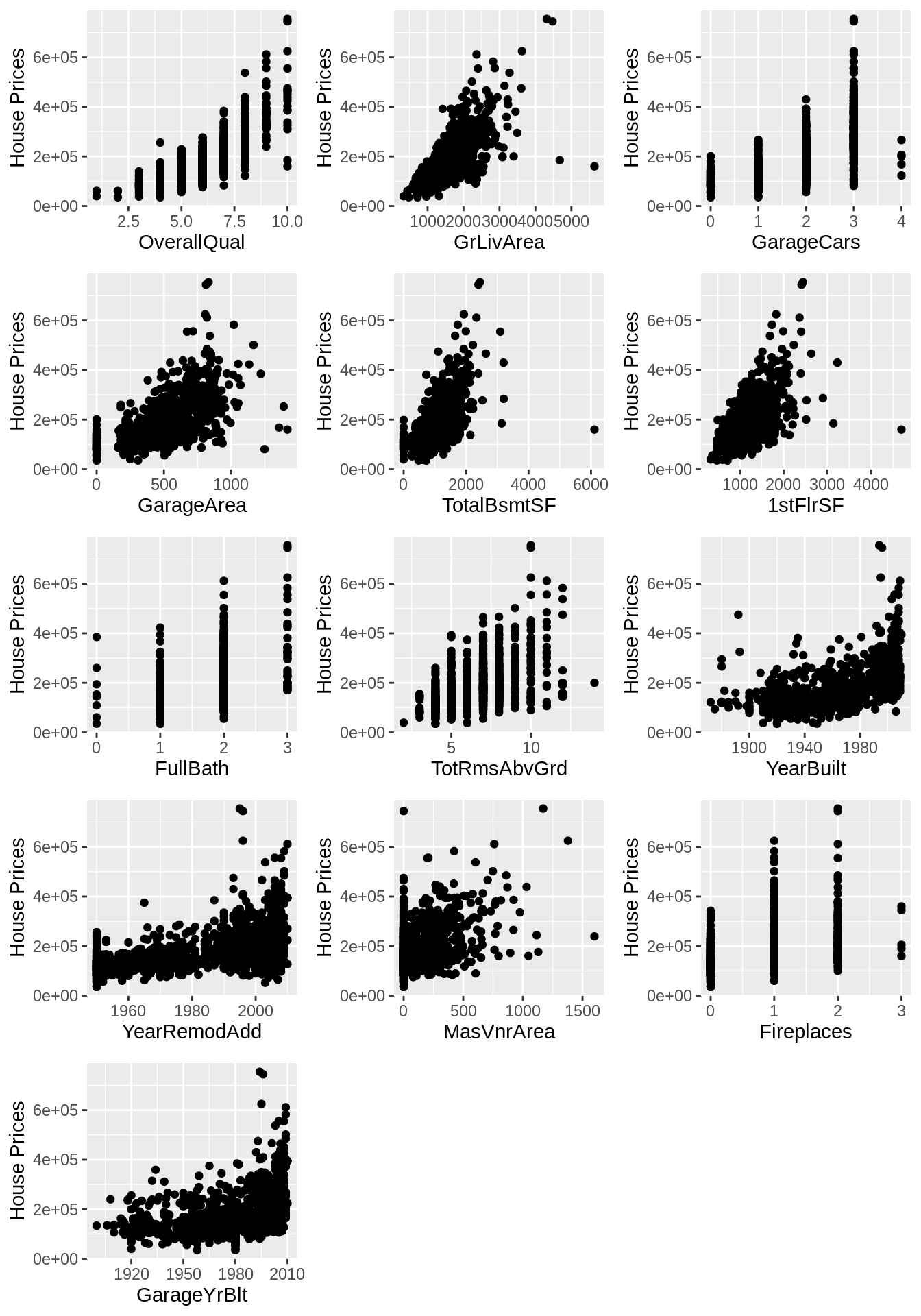
58.2.2 Explore & Handle Categorical Columns
Compute and show the proportions of missing values for each feature.
# show proportions of missing values
missing_col <- colSums(is.na(df[,cat_fea]))/dim(df)[1]
missing_col <- missing_col[missing_col > 0] %>% sort(decreasing = TRUE)
missing_col
## PoolQC MiscFeature Alley Fence FireplaceQu GarageType
## 0.9952054795 0.9630136986 0.9376712329 0.8075342466 0.4726027397 0.0554794521
## GarageFinish GarageQual GarageCond BsmtExposure BsmtFinType2 BsmtQual
## 0.0554794521 0.0554794521 0.0554794521 0.0260273973 0.0260273973 0.0253424658
## BsmtCond BsmtFinType1 MasVnrType Electrical
## 0.0253424658 0.0253424658 0.0054794521 0.0006849315Categorical features are usually more tricky because NA might not mean “unknown”. According to the data description, only “MasVnrType” and “Electrical” truly have “NA” as missing values, the NAs in other features just mean “None”. Another thing to note is, even though some categorical features have large portions of missing values, we cannot just delete the columns like how we handle numeric data. Sometimes, missing values could be super informative (for example, the mean house prices corresponding to the missing values of a feature is significantly higher than the rest of classes of that feature). Therefore, we should visualize missing values as an explicit class, and then decide on whether to drop the column or make missing values an indicator column. For features with few missing values, we can just fill NAs with mode.
# Find the mode for each feature
df %>% group_by_at('MasVnrType') %>% count()
## # A tibble: 5 × 2
## # Groups: MasVnrType [5]
## MasVnrType n
## <chr> <int>
## 1 BrkCmn 15
## 2 BrkFace 445
## 3 None 864
## 4 Stone 128
## 5 <NA> 8
df %>% group_by_at('Electrical') %>% count()## # A tibble: 6 × 2
## # Groups: Electrical [6]
## Electrical n
## <chr> <int>
## 1 FuseA 94
## 2 FuseF 27
## 3 FuseP 3
## 4 Mix 1
## 5 SBrkr 1334
## 6 <NA> 1
df[is.na(df['MasVnrType']), 'MasVnrType'] <- 'None'
df[is.na(df['Electrical']), 'Electrical'] <- 'SBrkr'
df[is.na(df)] <- 'None'
missing_col <- colSums(is.na(df[,cat_fea]))/dim(df)[1]
missing_col[missing_col > 0] %>% sort(decreasing = TRUE) # always check whether all NAs have been filled
## named numeric(0)Most models do not handle categorical features as is, and therefore we need to transform our categorical data into numeric data in a meaningful manner. There are three frequently used strategies:
- One-hot Encoding: transform each class of the categorical feature into a binary feature. This method works well for nominal features with low cardinality. One-hot might not work well for linear models because it causes multi-collinearity which breaks the assumption of independent features.
- Ordinal Encoding: transform each class of the ordinal categorical feature into an integer. The order of assigning integers should follow the internal order. For example, assign 1 to poor, 2 to average, 3 to good. When there are a lot of ordinal features with different sets of levels, this method could be tedious because we need to specify the internal order for each feature.
- Target Encoding: replace each class of the categorical feature with the mean of labels corresponding to that class. This method applies to all types of categorical features, especially good for categorical features with high cardinality.
House price dataset is a typical dataset with various categorical features. If we use one-hot, it will dramatically increase the dimension of our dataset. Since we have too many ordinal features with different set of levels, ordinal encoding is also not a good idea. Therefore, we can use target encoding here, which gives meaningful orders without causing multi-colinearity or increasing dimension. Moreover, since we have too many categorical features, it is hard to choose which features to visualize. If we use target encoding to transform features, we could choose and visualize categorical features just like how we handle numeric data.
target_encoder <- function(df, feature) { # feature input in string format
  fea = paste(feature, 'target', sep = '_')
  df1 <- df %>% group_by_at(feature) %>%
    summarise(n = mean(SalePrice)) %>%
    rename_with(.fn = function(x) fea, .cols = n) # rename encoded features
  df2 <- left_join(df, df1)
  df2 <- select_if(df2, names(df2) != feature) # drop original features
  return(df2)
}

for (i in cat_fea) {
  suppressMessages(df <- target_encoder(df, i)) # to avoid message of "joining by.."
}

str(df)
## tibble [1,460 × 79] (S3: tbl_df/tbl/data.frame)
## $ MSSubClass : num [1:1460] 60 20 60 70 60 50 20 60 50 190 ...
## $ LotArea : num [1:1460] 8450 9600 11250 9550 14260 ...
## $ OverallQual : num [1:1460] 7 6 7 7 8 5 8 7 7 5 ...
## $ OverallCond : num [1:1460] 5 8 5 5 5 5 5 6 5 6 ...
## $ YearBuilt : num [1:1460] 2003 1976 2001 1915 2000 ...
## $ YearRemodAdd : num [1:1460] 2003 1976 2002 1970 2000 ...
## $ MasVnrArea : num [1:1460] 196 0 162 0 350 0 186 240 0 0 ...
## $ BsmtFinSF1 : num [1:1460] 706 978 486 216 655 ...
## $ BsmtFinSF2 : num [1:1460] 0 0 0 0 0 0 0 32 0 0 ...
## $ BsmtUnfSF : num [1:1460] 150 284 434 540 490 64 317 216 952 140 ...
## $ TotalBsmtSF : num [1:1460] 856 1262 920 756 1145 ...
## $ 1stFlrSF : num [1:1460] 856 1262 920 961 1145 ...
## $ 2ndFlrSF : num [1:1460] 854 0 866 756 1053 ...
## $ LowQualFinSF : num [1:1460] 0 0 0 0 0 0 0 0 0 0 ...
## $ GrLivArea : num [1:1460] 1710 1262 1786 1717 2198 ...
## $ BsmtFullBath : num [1:1460] 1 0 1 1 1 1 1 1 0 1 ...
## $ BsmtHalfBath : num [1:1460] 0 1 0 0 0 0 0 0 0 0 ...
## $ FullBath : num [1:1460] 2 2 2 1 2 1 2 2 2 1 ...
## $ HalfBath : num [1:1460] 1 0 1 0 1 1 0 1 0 0 ...
## $ BedroomAbvGr : num [1:1460] 3 3 3 3 4 1 3 3 2 2 ...
## $ KitchenAbvGr : num [1:1460] 1 1 1 1 1 1 1 1 2 2 ...
## $ TotRmsAbvGrd : num [1:1460] 8 6 6 7 9 5 7 7 8 5 ...
## $ Fireplaces : num [1:1460] 0 1 1 1 1 0 1 2 2 2 ...
## $ GarageYrBlt : num [1:1460] 2003 1976 2001 1998 2000 ...
## $ GarageCars : num [1:1460] 2 2 2 3 3 2 2 2 2 1 ...
## $ GarageArea : num [1:1460] 548 460 608 642 836 480 636 484 468 205 ...
## $ WoodDeckSF : num [1:1460] 0 298 0 0 192 40 255 235 90 0 ...
## $ OpenPorchSF : num [1:1460] 61 0 42 35 84 30 57 204 0 4 ...
## $ EnclosedPorch : num [1:1460] 0 0 0 272 0 0 0 228 205 0 ...
## $ 3SsnPorch : num [1:1460] 0 0 0 0 0 320 0 0 0 0 ...
## $ ScreenPorch : num [1:1460] 0 0 0 0 0 0 0 0 0 0 ...
## $ PoolArea : num [1:1460] 0 0 0 0 0 0 0 0 0 0 ...
## $ MiscVal : num [1:1460] 0 0 0 0 0 700 0 350 0 0 ...
## $ MoSold : num [1:1460] 2 5 9 2 12 10 8 11 4 1 ...
## $ YrSold : num [1:1460] 2008 2007 2008 2006 2008 ...
## $ SalePrice : num [1:1460] 208500 181500 223500 140000 250000 ...
## $ MSZoning_target : num [1:1460] 191005 191005 191005 191005 191005 ...
## $ Street_target : num [1:1460] 181131 181131 181131 181131 181131 ...
## $ Alley_target : num [1:1460] 183452 183452 183452 183452 183452 ...
## $ LotShape_target : num [1:1460] 164755 164755 206102 206102 206102 ...
## $ LandContour_target : num [1:1460] 180184 180184 180184 180184 180184 ...
## $ Utilities_target : num [1:1460] 180951 180951 180951 180951 180951 ...
## $ LotConfig_target : num [1:1460] 176938 177935 176938 181623 177935 ...
## $ LandSlope_target : num [1:1460] 179957 179957 179957 179957 179957 ...
## $ Neighborhood_target : num [1:1460] 197966 238773 197966 210625 335295 ...
## $ Condition1_target : num [1:1460] 184495 142475 184495 184495 184495 ...
## $ Condition2_target : num [1:1460] 181169 181169 181169 181169 181169 ...
## $ BldgType_target : num [1:1460] 185764 185764 185764 185764 185764 ...
## $ HouseStyle_target : num [1:1460] 210052 175985 210052 210052 210052 ...
## $ RoofStyle_target : num [1:1460] 171484 171484 171484 171484 171484 ...
## $ RoofMatl_target : num [1:1460] 179804 179804 179804 179804 179804 ...
## $ Exterior1st_target : num [1:1460] 213733 149422 213733 149842 213733 ...
## $ Exterior2nd_target : num [1:1460] 214432 149803 214432 161329 214432 ...
## $ MasVnrType_target : num [1:1460] 204692 156958 204692 156958 204692 ...
## $ ExterQual_target : num [1:1460] 231634 144341 231634 144341 231634 ...
## $ ExterCond_target : num [1:1460] 184035 184035 184035 184035 184035 ...
## $ Foundation_target : num [1:1460] 225230 149806 225230 132291 225230 ...
## $ BsmtQual_target : num [1:1460] 202688 202688 202688 140760 202688 ...
## $ BsmtCond_target : num [1:1460] 183633 183633 183633 213600 183633 ...
## $ BsmtExposure_target : num [1:1460] 165652 257690 192790 165652 206643 ...
## $ BsmtFinType1_target : num [1:1460] 235414 161573 235414 161573 235414 ...
## $ BsmtFinType2_target : num [1:1460] 184695 184695 184695 184695 184695 ...
## $ Heating_target : num [1:1460] 182021 182021 182021 182021 182021 ...
## $ HeatingQC_target : num [1:1460] 214914 214914 214914 156859 214914 ...
## $ CentralAir_target : num [1:1460] 186187 186187 186187 186187 186187 ...
## $ Electrical_target : num [1:1460] 186811 186811 186811 186811 186811 ...
## $ KitchenQual_target : num [1:1460] 212116 139963 212116 212116 212116 ...
## $ Functional_target : num [1:1460] 183429 183429 183429 183429 183429 ...
## $ FireplaceQu_target : num [1:1460] 141331 205723 205723 226351 205723 ...
## $ GarageType_target : num [1:1460] 202893 202893 202893 134091 202893 ...
## $ GarageFinish_target : num [1:1460] 202069 202069 202069 142156 202069 ...
## $ GarageQual_target : num [1:1460] 187490 187490 187490 187490 187490 ...
## $ GarageCond_target : num [1:1460] 187886 187886 187886 187886 187886 ...
## $ PavedDrive_target : num [1:1460] 186434 186434 186434 186434 186434 ...
## $ PoolQC_target : num [1:1460] 180405 180405 180405 180405 180405 ...
## $ Fence_target : num [1:1460] 187597 187597 187597 187597 187597 ...
## $ MiscFeature_target : num [1:1460] 182046 182046 182046 182046 182046 ...
## $ SaleType_target : num [1:1460] 173402 173402 173402 173402 173402 ...
## $ SaleCondition_target: num [1:1460] 175202 175202 175202 146527 175202 ...Since all categorical features have been transformed into numeric features, we could visualize them in the same way as plotting numeric features.
for (i in 1:length(cat_fea)) {
  cat_fea[i] <- local({
    i <- i
    paste(cat_fea[i],'target',sep='_') # update categorical feature list
  })
}

corr <- cor(df[,append(cat_fea, label)])[,label]
corr <- corr[order(abs(corr), decreasing = TRUE)]
imp_num_fea <- names(corr[abs(corr)>0.4])
imp_num_fea <- imp_num_fea[imp_num_fea != label]

p <- list()
for (i in 1:length(imp_num_fea)) {
  p[[i]] <- local({
    i <- i
    ggplot() +
    geom_point(aes(x=unlist(df[,imp_num_fea[i]]), y=unlist(df[label]))) +
    xlab(imp_num_fea[i]) +
    ylab("House Prices")
  })
}
grid.arrange(grobs = p, ncol = 3)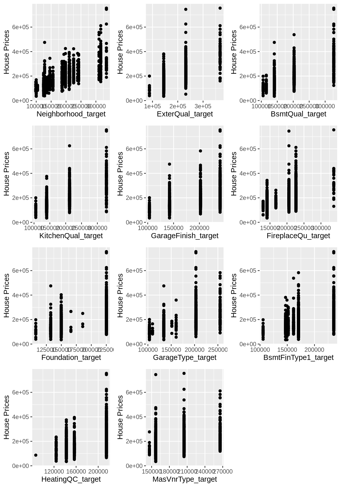
Finally All missing values have been filled, and all categorical features have been transformed. Now we are ready for modeling!
Note:
I did not remove any outliers here because it is not very reasonable to do that for such a small dataset. Moreover, even though we remove a few “outliers”, it would usually have little impact on model performance. The right way is just to keep all the data and run a model first. If there are certain predictions with dramatically higher errors, then we go into the data again and try to see if there are any outliers we should remove.
I did not scale the data here. Firstly, scaling is not needed for every model. For tree models, scaling just does not matter at all. However, for distance-based models, scaling might reduce training time, boost interpretability of feature importance, and improve accuracy/reduce error.