10 Introduction to Time Series
Parth Gupta (pg2677)
I am writing a tutorial for time series forecasting and I will be covering all the classical techniques to do time series forecasting.
10.1 Motivation,
Modeling temporal processes has always been one of the most important problems. Because it has a wide variety of applications, ranging from stock price prediction to weather forecasting to forecasting web traffic on a website.
We have three types of temporal data,
Time Series
Panel
Cross Sectional
In time series data we have one individual which is observed at different time steps. In Panel data we have multiple individuals that are observed at different time steps. In Cross sectional data we have different individuals observed at same time step.
Time series analysis comprises methods for analyzing time series data in order to extract meaningful statistics and other characteristics of the data. Time series forecasting is the use of a model to predict future values based on previously observed values. Time series forecasting is very useful because it has a lot of real life applications.
Visualizing a time series data is very important because then we will be able to get a much better understanding of the underlying patterns in the data. Like the trends if there is an increase or decrease in price of an item with time, seasonal changes like people watch movies more on weekends. How far is the prediction from the actual truth.
df <-births <- scan("http://robjhyndman.com/tsdldata/data/nybirths.dat")
data <- df[1:72]
future <- df[73:84]
print(data)
## [1] 26.663 23.598 26.931 24.740 25.806 24.364 24.477 23.901 23.175 23.227
## [11] 21.672 21.870 21.439 21.089 23.709 21.669 21.752 20.761 23.479 23.824
## [21] 23.105 23.110 21.759 22.073 21.937 20.035 23.590 21.672 22.222 22.123
## [31] 23.950 23.504 22.238 23.142 21.059 21.573 21.548 20.000 22.424 20.615
## [41] 21.761 22.874 24.104 23.748 23.262 22.907 21.519 22.025 22.604 20.894
## [51] 24.677 23.673 25.320 23.583 24.671 24.454 24.122 24.252 22.084 22.991
## [61] 23.287 23.049 25.076 24.037 24.430 24.667 26.451 25.618 25.014 25.110
## [71] 22.964 23.981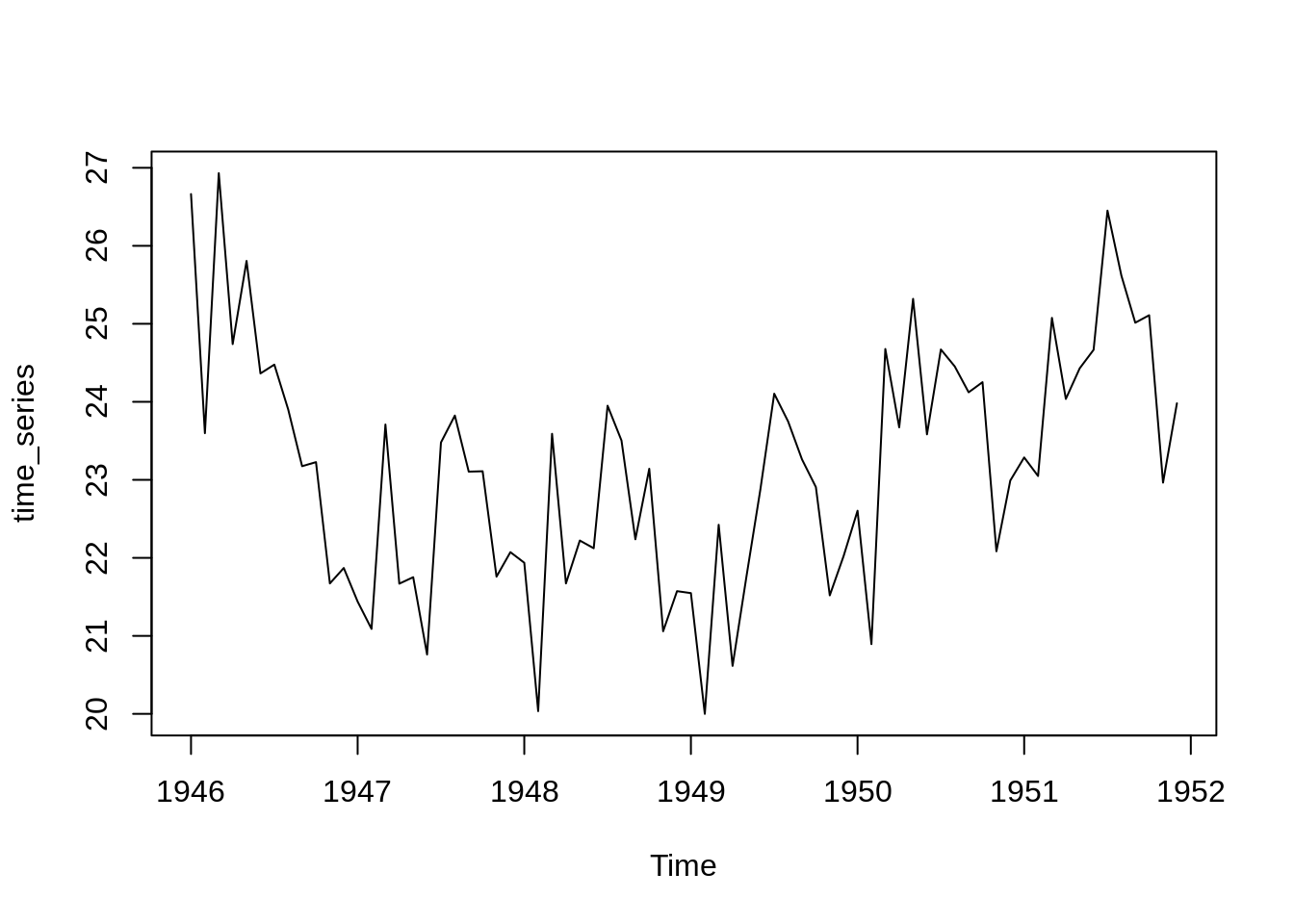
I am using the birth per month dataset. I will tune all the parameters of different models based on the training period from Jan 1946 to Dec 1951. I will forecast for the next year. We generally use Mean Absolute Percentage Error or Root Mean Squared Error to evaluate the model.
$$
MAPE = _{i = 0}^{N}|( - y_i)|/ y_i\
RMSE = (_{i = 0}^{N}( - y_i)^2/ N)^{1/2}
$$

Every time series has three components, trends, seasonality and residuals
Time Series = Trend + Seasonality + Residuals
Trend, it refers to the overall general direction of the data, obtained ignoring any short term effects such as seasonal variations or noise.
Seasonality, it refers to periodic fluctuations that are repeated throughout all the time series period.
Residuals, it refers to the left part after trend and seasonality.
monthplot(time_series)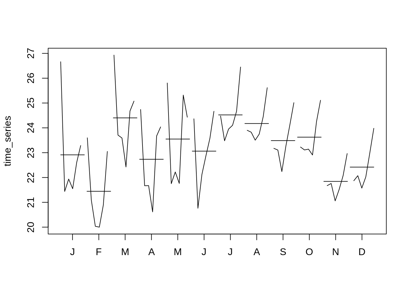
seasonplot(time_series)
In these plots I am trying to visualize the seasonality aspect of the time series data. I have plotted the data for each month for whole training period.
10.2 Stationary Time Series
Stationarity is one of the most important concepts in time series forecasting. A stationary time series is one whose properties do not depend on the time at which the series is observed. Thus, time series with trends, or with seasonality, are not stationary — the trend and seasonality will affect the value of the time series at different times. On the other hand, a white noise series is stationary — it does not matter when you observe it, it should look much the same at any point in time.
Differencing is the process of computing the differences between consecutive observations.
We apply log transformations to stabilise the variance of a time series. Differencing can also help in stabilising the mean of a time series by removing changes in the level of a time series, and therefore eliminating (or reducing) trend and seasonality. There are also some tests to check stationarity of a time series.
10.3 HoltWinters model,
This model has three parameters alpha, beta and gamma.
alpha: it refers to the “base value”. Higher alpha puts more weight on the most recent observations.
beta: it corresponds to the “trend value”. Higher beta means the trend slope is more dependent on recent trend slopes.
gamma: it weighs the “seasonal component”. Higher gamma puts more weighting on the most recent seasonal cycles.
The mathematical formulation is as follows,
$$ {y}{t+h|t} = l_t + hb_t + s{t+h-m(k+1)} \
l_t = (y_t - s_{t-m}) + (1- )*(l_{t-1} + b_{t-1})\
b_t = ^* (l_t - l_{t-1}) + (1-^*)b_{t-1}\
s_t = (y_t - l_{t-1} - b_{t-1}) + (1-)s_{t-m} $$
# simple exponential - models level
fit_1 <- HoltWinters(time_series, beta=FALSE, gamma=FALSE)
f1 = forecast(fit_1, 12)
plot(forecast(fit_1, 12))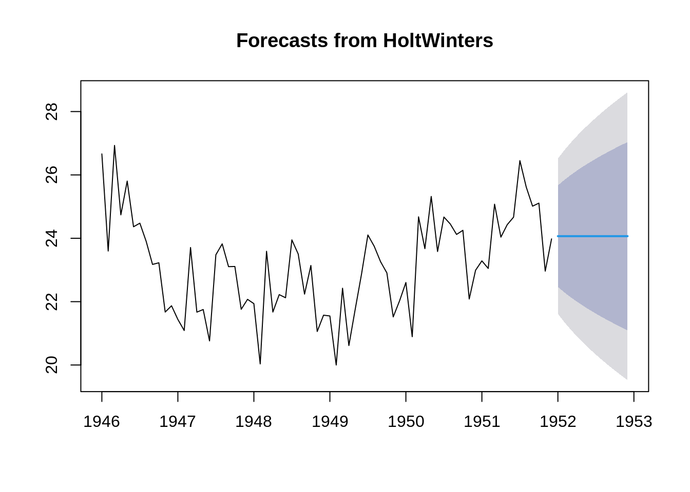
Let’s start with the simplest model, In this model we will forecast all the future value as the last value only, i.e.
y[t+i] = y[t], where i>=1 and t is the last time step in our training period.
$$
_{T+i} = y_T \ i>=1 $$
# double exponential - models level and trend
fit_2 <- HoltWinters(time_series, gamma=FALSE)
f2 = forecast(fit_2, 12)
plot(forecast(fit_2, 12))
Now we can set beta to non zero value so that we can account for trends, In this model we will forecast all the future value as the last value + trend.
# triple exponential - models level, trend, and seasonal components
fit_3 <- HoltWinters(time_series)
f3 = forecast(fit_3, 12)
plot(forecast(fit_3, 12))
Finally, we will set all the three parameters, alpha, beta and gamma to non zero values to account for trend and seasonality both.
Naturally, this model performs better than previous two models.
# Automated forecasting using an exponential model
fit_4 <- ets(time_series)
f4 = forecast(fit_4, 12)
plot(forecast(fit_4, 12))
10.4 Exponential Smooting
In this model, we assign weights to the past observations and we decrease them exponentially as we go back in time. This model ensures to give more weights to the recent observations and less and less weights to older observations
$$ {T+1|T} = y_T + (1-)* y{t-1} + (1-)^2 *y_{t-2} + …..\
{T+1|T} = {j = 0}{T-1}(1-)jy_{T-j} + (1-)^Tl_0 $$
10.5 ARIMA model,
ARIMA stands for Auto Regressive Integrated Moving Average. It is a generalization of the simpler AutoRegressive Moving Average and adds the notion of integration. Let’s look at each term individually.
AR: Autoregression. it refers to any model that predicts the future values by using past observations.
I: Integrated. We use the concept of differencing of raw observations (e.g. subtracting an observation from an observation at the previous time step) in order to make the time series stationary.
MA: Moving Average. it refers to any model that uses the dependency between an observation and a residual error from a moving average model applied to lagged observations.
We need all three parameters to define the model. We use the notation ARIMA(p,d,q).
The parameters of the ARIMA model are defined as follows:
p: The number of lag observations included in the model, also called the lag order. d: The number of times that the raw observations are differenced, also called the degree of differencing. q: The size of the moving average window, also called the order of moving average.
If there is a seasonal effect then, it is generally considered better to use a SARIMA (seasonal ARIMA) model than to increase the order of the AR or MA parts of the model.
#using an ARIMA model
fit_5 <- Arima(time_series, order = c(10, 1, 1))
f5 = forecast(fit_5, 12)
plot(forecast(fit_5, 12))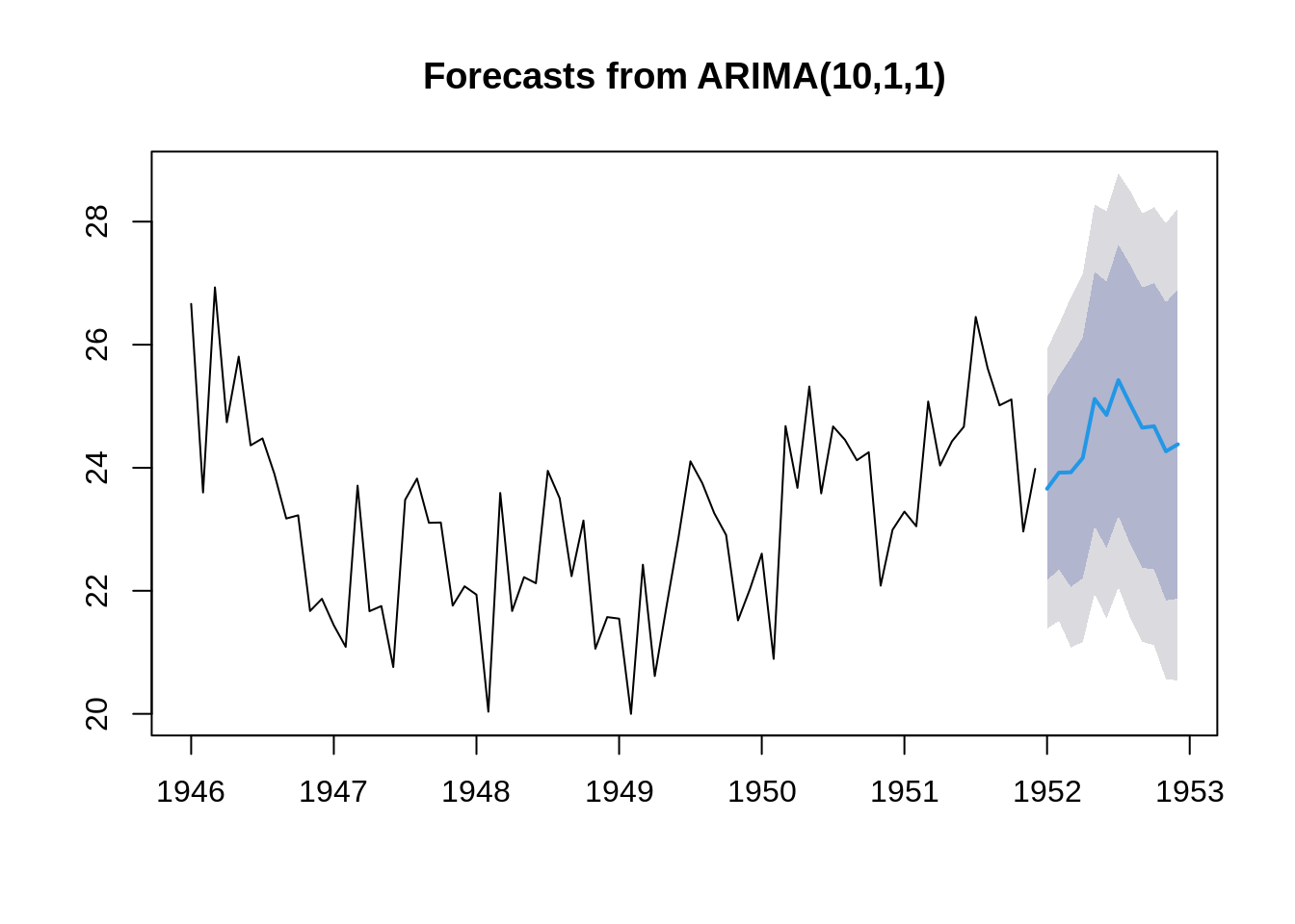
#using an ARIMA model
acf(time_series)
pacf(time_series)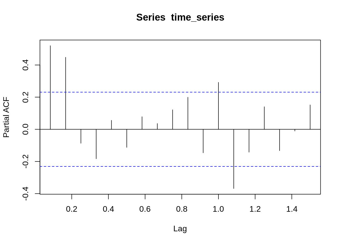
Now, it is very difficult to choose values of p, q so we can use Autocorrelation function (ACF), and Partial autocorrelation function (PACF) plots of the series to determine the order of AR and/ or MA terms.
The autocorrelation function (ACF) is a technique that we can use to identify how correlated the values in a time series are with each other. The ACF plots the correlation coefficient against the lag. A lag corresponds to a certain point in time after which we observe the first value in the time series.
Partial autocorrelation is a statistical measure that captures the correlation between two variables after controlling for the effects of other variables.
# Forecasting using an ARIMA model
fit_6 <- auto.arima(time_series)
f6 = forecast(fit_6, 12)
plot(forecast(fit_6, 12))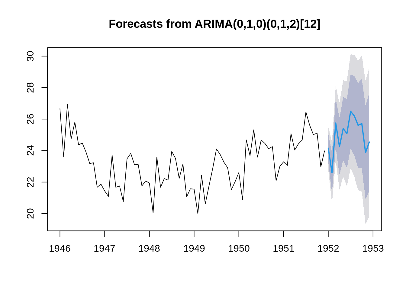
Now, we can use another implementation of ARIMA in R i.e the auto.arima() function which uses a variation of the Hyndman-Khandakar algorithm (Hyndman & Khandakar, 2008). It combines unit root tests, minimisation of the AICc and MLE to obtain an ARIMA model.
rmse_1 = accuracy(forecast(fit_1))[2]
rmse_2 = accuracy(forecast(fit_2))[2]
rmse_3 = accuracy(forecast(fit_3))[2]
rmse_4 = accuracy(forecast(fit_4))[2]
rmse_5 = accuracy(forecast(fit_5))[2]
rmse_6 = accuracy(forecast(fit_6))[2]
rmse = c(rmse_1, rmse_2, rmse_3, rmse_4, rmse_5, rmse_6)

barplot(rmse, main="RMSE Plot", xlab="Models", names.arg = c("HW_1", "HW_2", "HW_3", "ETS", "ARIMA", "Auto ARIMA"))
MAPE_1 = accuracy(forecast(fit_1))[5]
MAPE_2 = accuracy(forecast(fit_2))[5]
MAPE_3 = accuracy(forecast(fit_3))[5]
MAPE_4 = accuracy(forecast(fit_4))[5]
MAPE_5 = accuracy(forecast(fit_5))[5]
MAPE_6 = accuracy(forecast(fit_6))[5]
MAPE = c(MAPE_1, MAPE_2, MAPE_3, MAPE_4, MAPE_5, MAPE_6)

barplot(MAPE, main="MAPE Plot", xlab="Models", names.arg = c("HW_1", "HW_2", "HW_3", "ETS", "ARIMA", "Auto ARIMA"))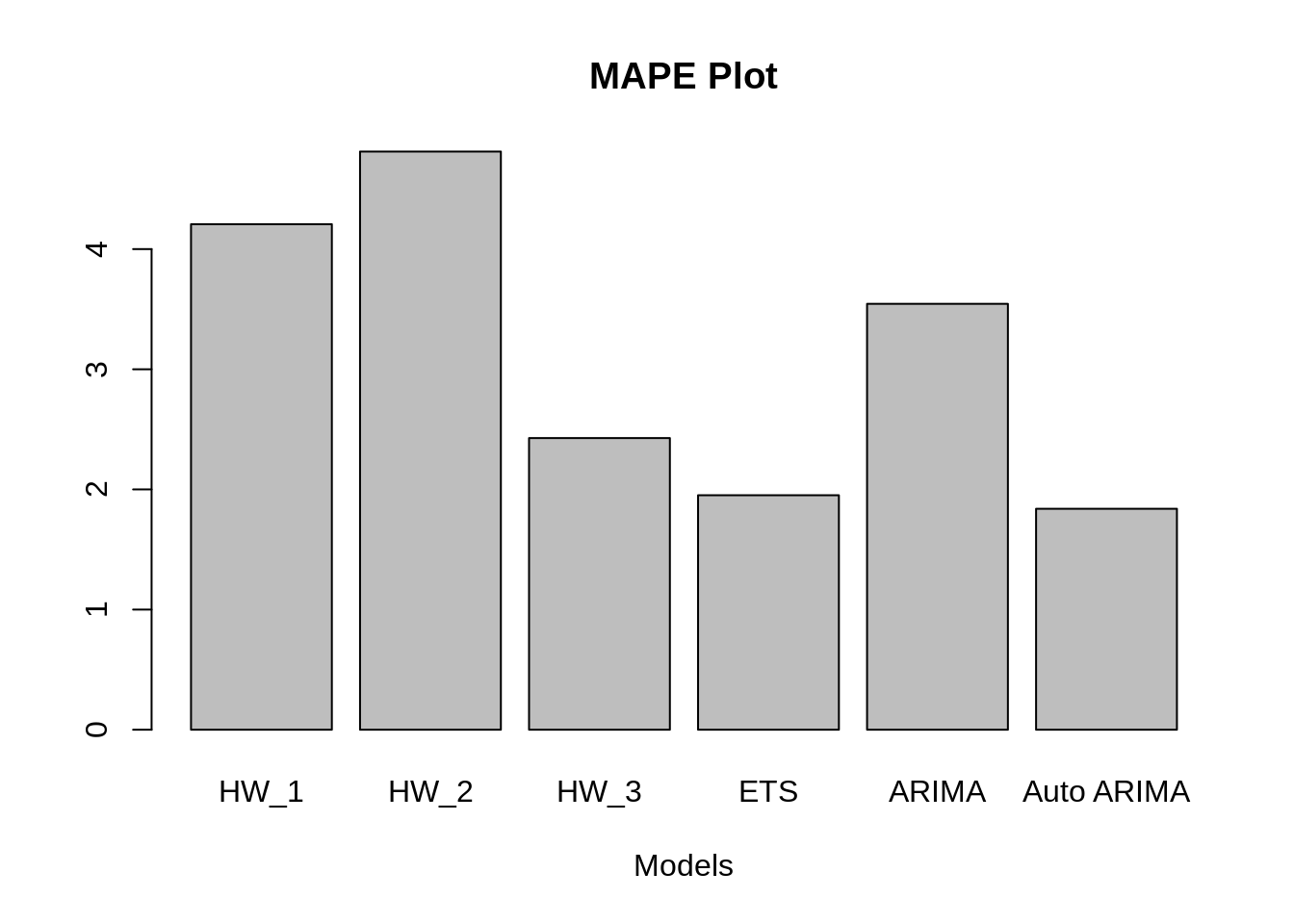
We, can clearly see from the above MAPE and RMSE bar plots that Auto ARIMA and ETS have performed the best followed by Holt Winter model with non zero alpha, beta and gamma.
References,
Hyndman, R.J., & Athanasopoulos, G. (2018) Forecasting: principles and practice, 2nd edition, OTexts: Melbourne, Australia.OTexts.com/fpp2.
https://www.analyticsvidhya.com/blog/2018/02/time-series-forecasting-methods/