30 Interactive plot introduction
Yujie Zhou
library(ggplot2)
library(plotly)
library(gapminder)
library("tidyr")
library("heatmaply")
library(igraph)
library(networkD3)
Interactive plots are used widely in today’s data analysis.This tutorial will introduce four commonly used interactive plots: interactive bubble plot, interactive area plot, interactive heatmap, and interactive network. Unlike static plot, interactive plot can enable users to zoom in and out and give user a better use experience and simplify analysis process.
30.1 Interactive Bubble Plot:
A bubble plot is where a third dimension is added on a scatterplot. The size of each bubble represent the additional numeric variable.
We can draw the plot directly using “plotly” just right after we draw a bubble plot using “ggplot”. The following is an example to see how the number and lifespan of people in different nations are associated.
knitr::opts_chunk$set(warning = F, message = F)

head(gapminder)
## # A tibble: 6 × 6
## country continent year lifeExp pop gdpPercap
## <fct> <fct> <int> <dbl> <int> <dbl>
## 1 Afghanistan Asia 1952 28.8 8425333 779.
## 2 Afghanistan Asia 1957 30.3 9240934 821.
## 3 Afghanistan Asia 1962 32.0 10267083 853.
## 4 Afghanistan Asia 1967 34.0 11537966 836.
## 5 Afghanistan Asia 1972 36.1 13079460 740.
## 6 Afghanistan Asia 1977 38.4 14880372 786.
p <- gapminder %>%
  filter(year==1967) %>%
  ggplot( aes(x=gdpPercap, y=lifeExp, size=pop,color=continent)) +
  geom_point() +
  scale_x_log10() +
  theme_bw()

ggplotly(p)
While the interactive bubble plot show a positive relationship between GPD and human’s lifespan, it also gives an additional information on the number of people in each dot. However, the drawback of bubble plots will be it is hard to judge how the relationship between x and y variables and the their variables (polpulation size for this example).
30.2 Interactive Area Plot:
Area plot do not differ a lot from regular line graphs, but with two exceptions: 1. The area between the x-axis and each individual line is filled with some color 2. The x-axis must have zero value
Area plots use different colors to give users a good sense on how quantities have changed over time a period of time. However, users should carefully use area plots, because the overlapping areas of plots will hide some information and the area under each line is hard to percisely calculated by user just by looking at the graph.
knitr::opts_chunk$set(warning = F, message = F)
df <- read.csv("resources/interactive_plot_plotly_cheatsheet/StudentsPerformancePart.csv")
head(df)
## gender race.ethnicity parental.level.of.education lunch
## 1 female group B bachelor's degree standard
## 2 female group C some college standard
## 3 female group B master's degree standard
## 4 male group A associate's degree free/reduced
## 5 male group C some college standard
## 6 female group B associate's degree standard
## test.preparation.course math.score reading.score writing.score
## 1 none 72 72 74
## 2 completed 69 90 88
## 3 none 90 95 93
## 4 none 47 57 44
## 5 none 76 78 75
## 6 none 71 83 78
df %>%
  filter(gender == "female",race.ethnicity=="group B")%>%
  pivot_longer(
    cols = c('math.score','reading.score','writing.score'),
    names_to = "Subject",
    values_to = "score"
  ) %>%
  group_by(Subject, parental.level.of.education) %>%
  summarise(score = mean(score)) %>%
  mutate(parental.level.of.education = factor(parental.level.of.education,levels=c("associate's degree", "bachelor's degree", "high school", "master's degree", "some college", "some high school")))%>%
  mutate(parental.level.of.education = as.numeric(parental.level.of.education)) %>%
  ggplot(aes(x= parental.level.of.education ,y=score,fill=Subject))+
  geom_area(alpha = 0.7) +
  scale_fill_manual(values = c("#F6D7A7", "#C8E3D4", "#87AAAA")) +
  scale_x_continuous(breaks =1:6,labels = c("associate's degree", "bachelor's degree", "high school", "master's degree", "some college", "some high school"))+
  theme_minimal() -> p2

p2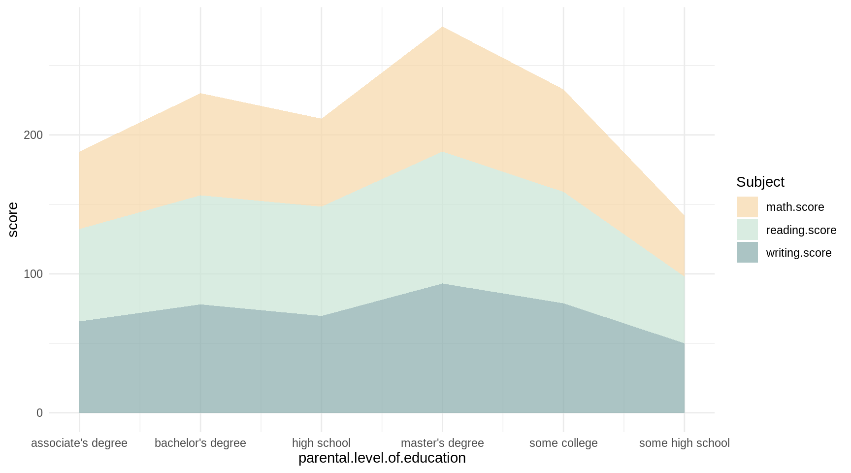
ggplotly(p2)We can easily see how the student mean performance for each subject associated with their parents’ educational background just by glancing at the area under each separate line.
30.3 Interactive Heatmap:
Heatmap is a very useful visualization tool on two-dimensional data to reveal patterns and correlations between by rows and columns. To be more easy-to-use, we will introduce interactive heatmap. As we already familiar with heatmap R package to draw a heatmap, we will use an useful R package “heatmaply” to build interactive cluster heatmap.
knitr::opts_chunk$set(warning = F, message = F)
data("mtcars")
heatmaply(mtcars, scale="column", Colv = NULL,col =  topo.colors(10),xlab="design", ylab="car type", main=" interactive heatmap")
mtcars is a collection fuel consumption corresponding to 10 automobile designs and 32 automobiles. It is noteworthy we should first do some data transformations, such as normalizing or percentizing to make variables more comparable. Normalizing the matrix is done using the scale argument. It can be applied to row or to column. Here the column option is chosen.
Passing NULL to Colv is because heatmap tends to reorder column by a clustering algorithm. Removing column dendrogram can enable users to compare between raw data.
It is also to good use terrain.color(), rainbow(), heat.colors(), topo.colors() or cm.colors() interchangeably by selecting different color palette for the heatmap.
Instead of vertically naming the x-axis as heatmap does, interactive heatmap will automatically rotate the name for x-axis values as names are too long to fit.
A more visual and user friendly tool,shinyHeatmaply, to create an interactive heatmap is invented byJonathan Sidi. To apply this tool, we can install ‘shinyHeatmaply’ R package, or, alternatively, run it through GitHub by entering “devtools::install_github(‘yonicd/shinyHeatmaply’)”. The output of heatmap from shinyHeatmaply will provide very detail parameter summaries.
30.4 Interactive Network
Network is consist of mainly two parts: nodes and edge. This graph reflect interrelationships between each note (i.e. entity). The advantage of using network is too include all important entities and analyze as a whole instead of see each entity separately. Two addtional packages we need to import for interactive network are igraph and networkD3. Let’s first see how igraph is used to plot a static network for a square matrix we generated ramdonly.
knitr::opts_chunk$set(warning = F, message = F)

set.seed(12345)
randomdf <- matrix(sample(0:3, 16, replace=TRUE), nrow=4)

output <- graph_from_adjacency_matrix(randomdf)
plot(output)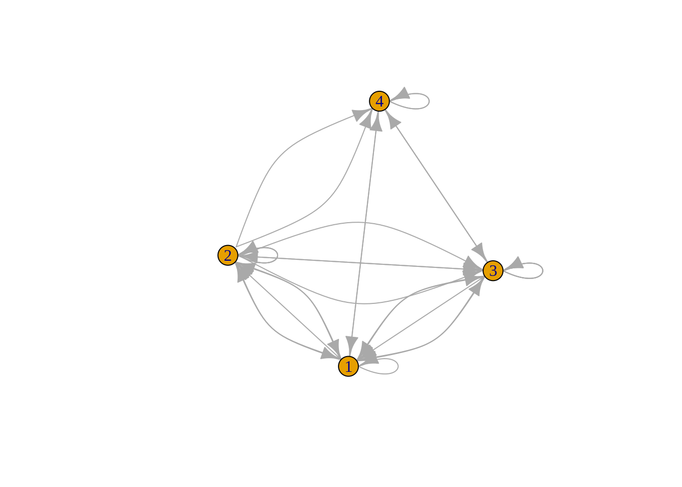
The arrow indicates the direction of relationship between two notes. For example, there is one relationship from 4 to 2, but there is no relationship from 2 to 4.
Now, let’s step to interactive networks. There is a very simple function: simpleNetwork which can generate interactive network in a handy way.
knitr::opts_chunk$set(warning = F, message = F)

data <- data.frame(
  from=c("A", "A", "B", "D", "C", "D", "E", "B", "C", "D", "K", "A", "M"),
  to=c("B", "E", "F", "A", "C", "A", "B", "Z", "A", "C", "A", "B", "K") #reference:https://www.r-graph-gallery.com/network-interactive.html
)
p <- simpleNetwork(data,height="50px", width="50px",
                   Source = 1,
                   Target = 2,
                   fontSize = 25,
                   linkColour = "#123",
                   nodeColour = "#F47E5E",
                   opacity = 0.9,
                   zoom = T)
p
Interactive network above we can rotate, zoom in, and zoom out the network and see it as a 3D layout. Compared to a static network, interactive network has a much better looking because when data gets bigger, it will avoid overlapping of links.