51 caret - a machine learning package turotial

Jiang Zhu and Xuechun Bai

Motivation: The motivation for this community contribution project is to introduce to classmates a package in R that can easily implement machine learning algorithms in few lines of code. As python users who commonly use the package scikit-learn to deploy machine laerning models, we strived to find a similar R package that has similar functions. While finding the resources online, we discovered that caret is a great package with neatly defined functions that create a easy-to use interface for machine learning algorithms, and at the same time, it has abundant machine learning models and preprocessing and model selection functions. However, we have not found any great tutorial or easy-to-read API’s for caret. Therefore, in this markdown file, we will illustrate how to use the caret package in a example-based manner. We eliminate the mathematics behind each model as much as possible to focus on the implementation of the algorithm in R. We will also demonstrate the results of our experiments of caret model on datasets with visualization tools.

library(caret)
library(tidyverse)
library(readr)
library(kernlab)
library(earth)
library(RANN)

51.1 Introduction and description of dataset

For the tutorial, we will use a data frame about Orange Juice which includes two orange juice brands, Citrus Hill (CH) and Minute Maid (MM) and selling information according to each brand. The URL of the dataset is : https://raw.githubusercontent.com/selva86/datasets/master/orange_juice_withmissing.csv, which contains 18 cloumns and 1070 rows.

The first column “Purchase” introduces brand of orange juice. the data contains weekly amount of purchase of the two brands (WeekofPurchase) with the store id (StoreID) where the orange juice was sold, and the price of the orange juice according to brand CH (PriceCH) and MM (PriceMM). The data also includes the discount (“DiscCH” and “DiscMM”), sale price(“SalePriceCH” and “SalePriceMM”) and other useful information about those two orange juice brands. The goal of our tutorial is to predict the customers’ preference between two brands when choosing to buy a orange juice, so we will only focusing on the “Purchase” for now.

Now let us firstly import the data, and state a briefly summary about this data:

# Import dataset
df <- read.csv('https://raw.githubusercontent.com/selva86/datasets/master/orange_juice_withmissing.csv')

# Structure of the dataframe
head(df)

##   Purchase WeekofPurchase StoreID PriceCH PriceMM DiscCH DiscMM SpecialCH
## 1       CH            237       1    1.75    1.99   0.00    0.0         0
## 2       CH            239       1    1.75    1.99   0.00    0.3         0
## 3       CH            245       1    1.86    2.09   0.17    0.0         0
## 4       MM            227       1    1.69    1.69   0.00    0.0         0
## 5       CH            228       7    1.69    1.69   0.00    0.0         0
## 6       CH            230       7    1.69    1.99   0.00    0.0         0
##   SpecialMM  LoyalCH SalePriceMM SalePriceCH PriceDiff Store7 PctDiscMM
## 1         0 0.500000        1.99        1.75      0.24     No  0.000000
## 2         1 0.600000        1.69        1.75     -0.06     No  0.150754
## 3         0 0.680000        2.09        1.69      0.40     No  0.000000
## 4         0 0.400000        1.69        1.69      0.00     No  0.000000
## 5         0 0.956535        1.69        1.69      0.00    Yes  0.000000
## 6         1 0.965228        1.99        1.69      0.30    Yes  0.000000
##   PctDiscCH ListPriceDiff STORE
## 1  0.000000          0.24     1
## 2  0.000000          0.24     1
## 3  0.091398          0.23     1
## 4  0.000000          0.00     1
## 5  0.000000          0.00     0
## 6  0.000000          0.30     0

51.2 Pre-processing

After importing the dataset, we need to separate data into training and testing sets. The training set is used as examples for machine learning models to learn generalize, and the test set is used to evaluate the preformance of our models. We can achieve this by using createDataPartition() in caret package.

createDataPartition(
  y,
  times,
  p,
  list
)

y specifies the column to which we will partition the data
times specifies how many times we will partition nthe data
p specifies the proportion to which we split the data
list is a boolean indicating whether we return a list

Here we set 70% of training set and 30% of testing set.

#set random seed to produce the same result
set.seed(1)

#use createDataPartition() function to get row of training. The input variable here is "Purchase" in df, and p = .7 implies the percentage of dataset we want to take. Here we set the training with 70%, so we let p equals to 0.7. Using List = F we are able to prevent the result as being a list instead of a dataframe.
rowOfTrain <- createDataPartition(df$Purchase, p=0.7, list=FALSE)

# create datasets for training and testing
train_df <- df[rowOfTrain,]
test_df <- df[-rowOfTrain,]

The next step is to clear or refill the missing values or NAs in the dataset. There are several ways of trasnformation such as fill the missing value into mean, mode or simply delete the row of missing values. Using caret package, we can apply the NAs to more practical values, which is to predict the missing values by other values that are listed in the dataset. The way caret package can do is to use preProcess() function to make k-Nearest Neighbors and use it with training set.

preProcess(
  data,
  method
)

data specifies the dataframe we want to apply the preprocessing
method is a string that specifies the method for preprocessing

Then we will get a Nearest model for perdicting the missing values. After that, we will use predict() to fill the missing values with our prediction.

# Create k-Nearest with training data using method = 'knnImpute'
knn_inputer <- preProcess(train_df, method='knnImpute')
knn_inputer

## Created from 727 samples and 18 variables
## 
## Pre-processing:
##   - centered (16)
##   - ignored (2)
##   - 5 nearest neighbor imputation (16)
##   - scaled (16)

# Import the prediction into missing values using function predict()
train_df <- predict(knn_inputer, newdata = train_df)

#Check the NAs in the training dataset
anyNA(train_df)

## [1] FALSE

From the result, we can see the prediction model has centered with 16 variables, ignored with 2 and was created from 825 samples and 18 variables. Then after importing the NAs by “predict” function, we then check if there are any missing values remaining in the dataset using angNA() function. The result of “FALSE” shows that the missing values are all replaced.

Another work the caret package can do is to transform the categorical variables into one-hot vectors to have a numerical representation of categorical variables. An one-hot vector is constructed as follows: suppose there are \(n\) classes of categorical variables. Then we represent each class \(i\) by a \(n\)-dimensional vector \(o_i\) such that \(o_i[i]=1\) and \(o_i[j]=0\) for all \(j\neq i\)

We can acheive the one-hot transformation using the dummyVars()

dummyVars(
  formula,
  data
)

formula repersents a way to inpute the data
data represents the dataframe

# define the one-hot encoding object
one_hot_encoder <- dummyVars(Purchase~., train_df)

# results after applying one-hot encoding
head(data.frame(predict(one_hot_encoder, train_df)))

##   WeekofPurchase   StoreID     PriceCH     PriceMM     DiscCH     DiscMM
## 1     -1.1406992 -1.267157 -1.16230500 -0.70167093 -0.4532457 -0.5650681
## 2     -1.0116414 -1.267157 -1.16230500 -0.70167093 -0.4532457  0.8702789
## 3     -0.6244679 -1.267157 -0.08909746  0.03485153  0.9895487 -0.5650681
## 4     -1.7859884 -1.267157 -1.74769093 -2.91123832 -0.4532457 -0.5650681
## 5     -1.7214595  1.327114 -1.74769093 -2.91123832 -0.4532457 -0.5650681
## 6     -1.5924017  1.327114 -1.74769093 -0.70167093 -0.4532457 -0.5650681
##    SpecialCH  SpecialMM     LoyalCH SalePriceMM SalePriceCH  PriceDiff Store7No
## 1 -0.4101973 -0.4461947 -0.24490422  0.08791265  -0.4606397  0.3276049        1
## 2 -0.4101973  2.2381700  0.08369962 -1.10522569  -0.4606397 -0.7838676        1
## 3 -0.4101973 -0.4461947  0.34658269  0.48562543  -0.8807610  0.9203903        1
## 4 -0.4101973 -0.4461947 -0.57350806 -1.10522569  -0.8807610 -0.5615731        1
## 5 -0.4101973 -0.4461947  1.25528731 -1.10522569  -0.8807610 -0.5615731        0
## 6 -0.4101973  2.2381700  1.28385285  0.08791265  -0.8807610  0.5498994        0
##   Store7Yes  PctDiscMM PctDiscCH ListPriceDiff      STORE
## 1         0 -0.5718037 -0.449862     0.2132873 -0.4419062
## 2         0  0.9396462 -0.449862     0.2132873 -0.4419062
## 3         0 -0.5718037  1.016257     0.1218262 -0.4419062
## 4         0 -0.5718037 -0.449862    -1.9817791 -0.4419062
## 5         1 -0.5718037 -0.449862    -1.9817791 -1.1401926
## 6         1 -0.5718037 -0.449862     0.7620539 -1.1401926

As we can see, the Store7.No and Store7.Yes represent the one-hot encoding. We will not actually apply it to the dataset because caret supports factor as the labels.

51.3 Model training

The machine learning models are defined and trained in caret by the train() function. It is the core function that masks all the tedious detail of the machine learning algorithms and provide a convenient and concise interface. The train() function has versions with different parameters:

# first version of train
model <- train(
  formula,
  data,
  method,
)

# second version of train
model <- train(
  x,
  y,
  method,
)

formula specifies the way we want to construct our model
data specifies the training data we want to use to construct the label
method is a string specifiying the model we want to apply to the data

The first version of the train function is recommended when we have all the data in a single dataframe. In another word, each column represents a feature \(x_i\) with one column represents \(y\). The second version of the train function is recommended when we have \(x\) and \(y\) as separate dataframes. In the following code, we will use the first version of train() on our prediction.

The method parameter can be specified conveniently by a string. By far there are 238 models supported by caret which can be found on https://topepo.github.io/caret/available-models.html. In this tutorial, we will illustrate and apply several common classification algorithms on our dataset.

One amazing feature of caret is that for almost all methods, it will automatically finds the best hyperparameters for the user.

51.3.1 K-nearest neighbors

k-nearest neighbor is the most intuitive classification algorithm. Given some positive \(k\) and some data \(x\), k-neigherest neighbor finds the k nearest neighbors in the training set based on the euclidian distance \[dist(x,x')=\sqrt{(x_1-x'_1)^2+(x_2-x'_2)^2+\cdots + (x_n-x'_n)^2}\] and classifies \(x\) as the class that contains the most nearst neighbors.

To implement such algorithm, we will specify the parameter method=knn

# training the knn model
knn_model <- train(
  Purchase ~.,
  train_df,
  method = "knn"
)

knn_model

## k-Nearest Neighbors 
## 
## 750 samples
##  17 predictor
##   2 classes: 'CH', 'MM' 
## 
## No pre-processing
## Resampling: Bootstrapped (25 reps) 
## Summary of sample sizes: 750, 750, 750, 750, 750, 750, ... 
## Resampling results across tuning parameters:
## 
##   k  Accuracy   Kappa    
##   5  0.7430519  0.4561180
##   7  0.7506511  0.4701385
##   9  0.7522812  0.4717872
## 
## Accuracy was used to select the optimal model using the largest value.
## The final value used for the model was k = 9.

51.3.2 Logistics Regression

logistics regression is linear model for binary classification, in another word, given features \(x_1,x_2,\cdots,x_n\), we want to predict \(y=\{0,1\}\). The model can be described by equation \[\hat{y}=\sigma(w_1\cdot x_1+w_2\cdot x_2+\cdots+w_n\cdot x_n)\] where the \(\sigma\) function is defined by \[\sigma(x)=\frac{1}{1+e^{-x}}\]

we hope that the logistics regression algorithm can find the optimal \(w_1,\cdots,w_n\) such that \(\hat{y}\) is as closed to the true label \(y\) as possible.

To implement such algorithm, we will specify the parameter method="glm":

# training the logistics regression model
lr_model <- train(
  Purchase ~.,
  train_df,
  method = "glm"
)

lr_model

## Generalized Linear Model 
## 
## 750 samples
##  17 predictor
##   2 classes: 'CH', 'MM' 
## 
## No pre-processing
## Resampling: Bootstrapped (25 reps) 
## Summary of sample sizes: 750, 750, 750, 750, 750, 750, ... 
## Resampling results:
## 
##   Accuracy   Kappa    
##   0.8219706  0.6207552

51.3.3 Support vector machine

support vector machine is a hyperplane that separates the input space into two subspaces. In the case when only we have \(x_1\) and \(x_2\), we want to draw a line that saparates the cartesian plane. The criteria for choosing such plane is the one that maximizes the distance to the closest data points from both classes. This gives rise to the optimization objective \[\max_{w,b}\frac{1}{\vert\vert w\vert\vert_2}\min_{x_i\in D}\vert w^Tx_i+b\vert,\quad \text{ s.t. }\forall i,\quad y_i(w^Tx_i+b)\ge 0 \] To implement such algorithm, we will specify the parameter method="svmRadial"

# training the support vector machine model, the library kernlab is needed to perform kernal transformation
svm_model <- train(
  Purchase ~.,
  train_df,
  method = "svmRadial"
)

svm_model

## Support Vector Machines with Radial Basis Function Kernel 
## 
## 750 samples
##  17 predictor
##   2 classes: 'CH', 'MM' 
## 
## No pre-processing
## Resampling: Bootstrapped (25 reps) 
## Summary of sample sizes: 750, 750, 750, 750, 750, 750, ... 
## Resampling results across tuning parameters:
## 
##   C     Accuracy   Kappa    
##   0.25  0.8126657  0.5977679
##   0.50  0.8143211  0.6016239
##   1.00  0.8123949  0.5975775
## 
## Tuning parameter 'sigma' was held constant at a value of 0.05934766
## Accuracy was used to select the optimal model using the largest value.
## The final values used for the model were sigma = 0.05934766 and C = 0.5.

51.3.4 Random Forest

The decision tree algorithm learns to predict the value of a target variable by learning simple decision rules inferred from the data features. The process for constructing the tree is to first select a root node \(x_i\) and a decision boundry \(b_i\). Then we recirsively select its children nodes and a corresponding decision threshold \(b\) such that it maximizes the information gain. Since different initialization produces different results, random forest aims to create multiple trees with different initialization and collectively ageraging the result that is produced by each individual decision trees

To implement such algorithm, we will specify the parameter method="earch"

# training the random forest model, the library earth is needed
rf_model <- train(
  Purchase ~.,
  train_df,
  method = "earth"
)

rf_model

## Multivariate Adaptive Regression Spline 
## 
## 750 samples
##  17 predictor
##   2 classes: 'CH', 'MM' 
## 
## No pre-processing
## Resampling: Bootstrapped (25 reps) 
## Summary of sample sizes: 750, 750, 750, 750, 750, 750, ... 
## Resampling results across tuning parameters:
## 
##   nprune  Accuracy   Kappa    
##    2      0.7958702  0.5634097
##   12      0.8095924  0.5959591
##   23      0.8081299  0.5933340
## 
## Tuning parameter 'degree' was held constant at a value of 1
## Accuracy was used to select the optimal model using the largest value.
## The final values used for the model were nprune = 12 and degree = 1.

51.4 Model prediction and evaluation

After we successfully train the models, it is time to evaluate them on the test set to validate if it is a good model. The key function to achieve this is the predict() function:

predict(
  object,
  newdata
)

To evaluate the models we have trained above, we can call the predict() function on each models:

# inpute the test data first
test_df <- predict(knn_inputer, test_df)

we can compute the confution matrix for each model:

Confusion matrix for the knn model:

knn_cm <- confusionMatrix(reference = factor(test_df$Purchase), data = predict(knn_model, test_df), mode='everything', positive='MM')

knn_cm$table

##           Reference
## Prediction  CH  MM
##         CH 169  30
##         MM  26  95

ggplot(data = data.frame(knn_cm$table), aes(x=Reference, y=Prediction))+
  geom_tile(aes(fill=Freq)) +
  scale_fill_gradient2(low="light blue", high="blue") +
  geom_text(aes(label=Freq)) +
  ggtitle("Confution matrix for KNN model")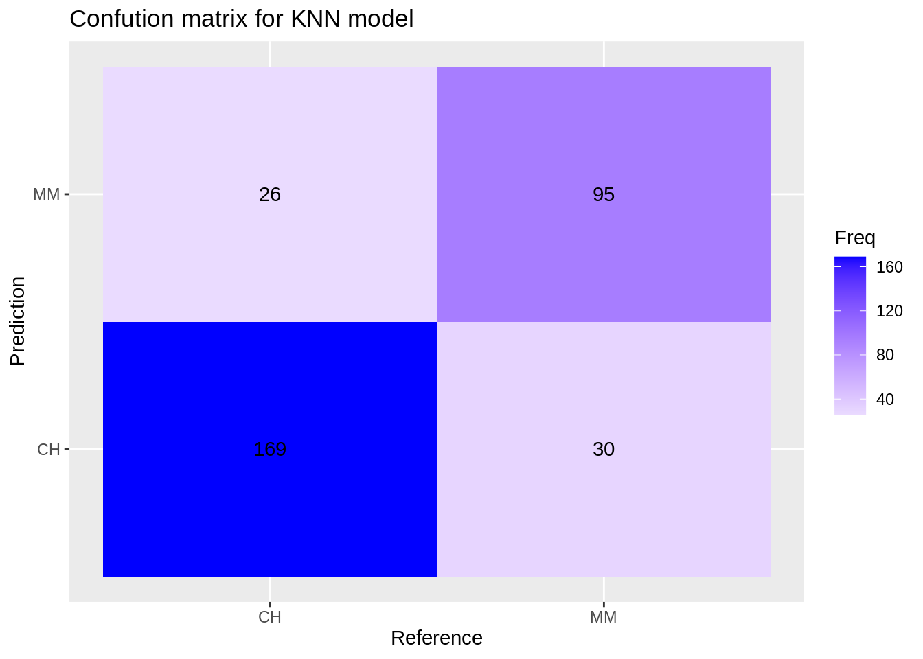

Confusion matrix for the logistics regression model:

lr_cm <- confusionMatrix(reference = factor(test_df$Purchase), data = predict(lr_model, test_df), mode='everything', positive='MM')

lr_cm$table

##           Reference
## Prediction  CH  MM
##         CH 164  20
##         MM  31 105

ggplot(data = data.frame(lr_cm$table), aes(x=Reference, y=Prediction))+
  geom_tile(aes(fill=Freq)) +
  scale_fill_gradient2(low="light blue", high="blue") +
  geom_text(aes(label=Freq)) +
  ggtitle("Confution matrix for Logistics Regression model")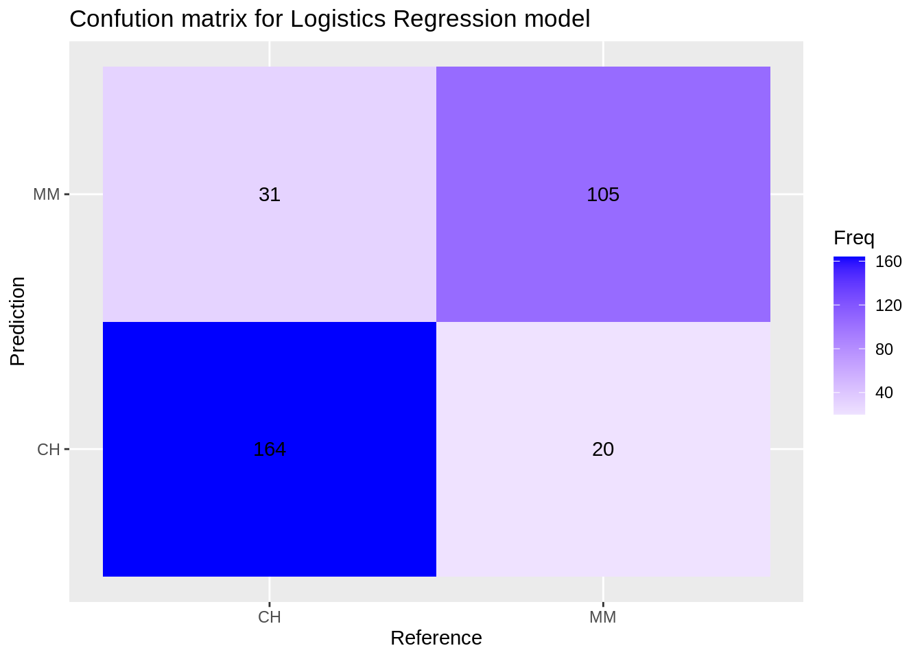

Confusion matrix for the svm model:

svm_cm <- confusionMatrix(reference = factor(test_df$Purchase), data = predict(svm_model, test_df), mode='everything', positive='MM')

svm_cm$table

##           Reference
## Prediction  CH  MM
##         CH 170  27
##         MM  25  98

ggplot(data = data.frame(svm_cm$table), aes(x=Reference, y=Prediction))+
  geom_tile(aes(fill=Freq)) +
  scale_fill_gradient2(low="light blue", high="blue") +
  geom_text(aes(label=Freq)) +
  ggtitle("Confution matrix for SVM model")

Confusion matrix for the random forest model:

rf_cm <- confusionMatrix(reference = factor(test_df$Purchase), data = predict(svm_model, test_df), mode='everything', positive='MM')

rf_cm$table

##           Reference
## Prediction  CH  MM
##         CH 170  27
##         MM  25  98

ggplot(data = data.frame(rf_cm$table), aes(x=Reference, y=Prediction))+
  geom_tile(aes(fill=Freq)) +
  scale_fill_gradient2(low="light blue", high="blue") +
  geom_text(aes(label=Freq)) +
  ggtitle("Confution matrix for random forest model")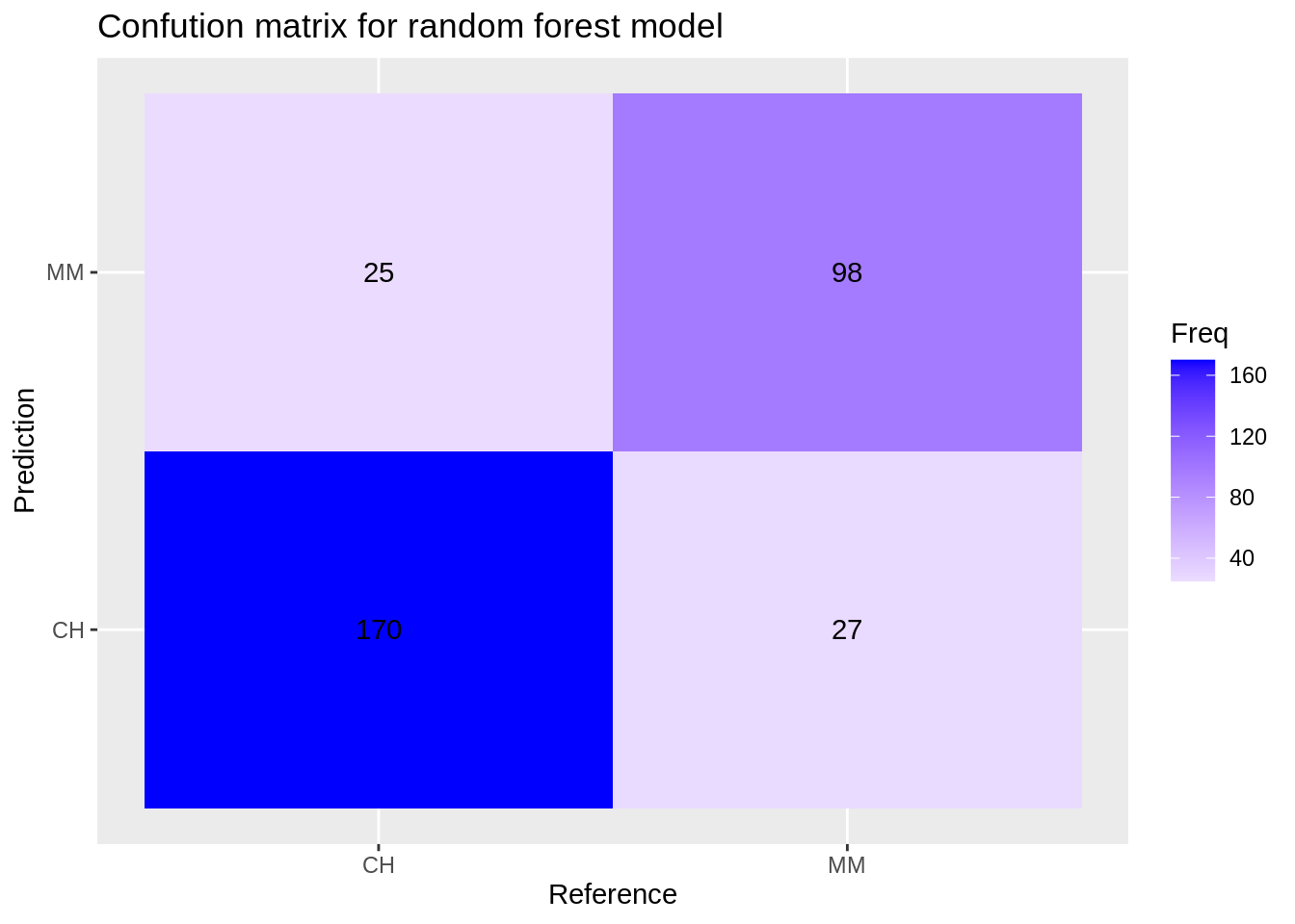

The caret package also provides a convenient function resamples() to compare the metric between models.

model_list <- list(KNN = knn_model, LR = lr_model, SVM = svm_model, RF = rf_model)

models_compare <- resamples(model_list)

summary(models_compare)

## 
## Call:
## summary.resamples(object = models_compare)
## 
## Models: KNN, LR, SVM, RF 
## Number of resamples: 25 
## 
## Accuracy 
##          Min.   1st Qu.    Median      Mean   3rd Qu.      Max. NA's
## KNN 0.7025090 0.7343173 0.7491166 0.7522812 0.7703180 0.8197880    0
## LR  0.7909408 0.8118081 0.8201439 0.8219706 0.8297101 0.8763636    0
## SVM 0.7620818 0.8013937 0.8172043 0.8143211 0.8239700 0.8525180    0
## RF  0.7750000 0.7906137 0.8058608 0.8095924 0.8230769 0.8625954    0
## 
## Kappa 
##          Min.   1st Qu.    Median      Mean   3rd Qu.      Max. NA's
## KNN 0.3824306 0.4294194 0.4604863 0.4717872 0.5098018 0.6148838    0
## LR  0.5476278 0.5914299 0.6196513 0.6207552 0.6368782 0.7459377    0
## SVM 0.4965787 0.5830797 0.6013610 0.6016239 0.6178862 0.6848073    0
## RF  0.5198789 0.5579644 0.5906583 0.5959591 0.6214686 0.7077705    0

As we can see that the random forest has the best performance on the dataset.

51.5 Reference

Caret Package – A Practical Guide to Machine Learning in R - Selva Prabhakaran: https://www.machinelearningplus.com/machine-learning/caret-package/#61howtotrainthemodelandinterprettheresults?

A basic tutorial of caret: the machine learning package in R - Rebecca Barter: https://www.rebeccabarter.com/blog/2017-11-17-caret_tutorial/

The caret Package - Max Kuhn: https://topepo.github.io/caret/index.html

50 Regression and Classification in R

52 Supervised Learning Tutorial