2 R Basics

So…there is soooo much to the world of R. Textbooks, cheatsheets, exercises, and other buzzwords full of resources you could go through. As of 2022-03-29, there are over 19000 packages on CRAN, the network through which R code and packages are distributed. It can be overwhelming. However, bear in mind that R is being used for a lot of different things, not all of which are relevant to EDAV.
In an effort to get everyone on the same page, here is a checklist of essentials so you can get up and running with this course. The best resources are scattered in different places online, so bear with links to various sites depending on the topic.
2.1 Top 10 Essentials Checklist
(r4ds = R for Data Science by Garrett Grolemund and Hadley Wickham, free online)
Install R (r4ds) – You need to have this installed but you won’t open the application since you’ll be working in RStudio. If you already installed R, make sure you’re current! The latest version of R (as of 2022-03-29) is R 4.1.3 “One Push-Up” released on 2022/03/10.
Install RStudio (r4ds) – Download the free, Desktop version for your OS. Working in this IDE will make working in R much more enjoyable. As with R, stay current. RStudio is constantly adding new features. The latest version (as of 2022-03-29) is 2022021+46.
Get comfortable with RStudio – In this chapter of Bruno Rodriguez’s Modern R with the Tidyverse, you’ll learn about panes, options, getting help, keyboard shortcuts, projects, add-ins, and packages. Be sure to try out:
- Do some math in the console
- Create an R Markdown file (
.Rmd) and render it to.html - Install some packages like
tidyverseorMASS
Another great option for learning the IDE: Watch Writing Code in RStudio (RStudio webinar)
Learn “R Nuts and Bolts” – Roger Peng’s chapter in R Programming will give you a solid foundation in the basic building blocks of R. It’s worth making the investing in understanding how R objects work now so they don’t cause you problems later. Focus on vectors and especially data frames; matrices and lists don’t come up often in data visualization. Get familiar with R classes: integer, numeric, character, and logical. Understand how factors work; they are very important for graphing.
Tidy up (r4ds) – Install the tidyverse, and get familiar with what it is. We will discuss differences between base R and the tidyverse in class.
Learn ggplot2 basics (r4ds) – In class we will study the grammar of graphics on which ggplot2 is based, but it will help to familiarize yourself with the syntax in advance. Avail yourself of the “Data Visualization with ggplot2” cheatsheet by clicking “Help” “Cheatsheets…” within RStudio.
Learn some RMarkdown – For this class you will write assignments in R Markdown (stored as
.Rmdfiles) and then render them into pdfs for submission. You can jump right in and open a new R Markdown file (File > New File > R Markdown…), and leave theDefault Output FormatasHTML. You will get a R Markdown template you can tinker with. Click the “knit” button and see what happens. For more detail, watch the RStudio webinar Getting Started with R MarkdownUse RStudio projects (r4ds) – If you haven’t already, drink the Kool-Aid. Make each problem set a separate project. You will never have to worry about
getwd()orsetwd()again because everything will just be in the right places.Or watch the webinar: “Projects in RStudio”
Learn the basic dplyr verbs for data manipulation (r4ds) – Concentrate on the main verbs:
filter()(rows),select()(columns),mutate(),arrange()(rows),group_by(), andsummarize(). Learn the pipe%>%operator.Know how to tidy your data – The
pivot_longer()function from the tidyr package – successor togather()– will help you get your data in the right form for plotting. More on this in class. Check out these super cool animations, which follow a data frame as it is transformed bytidyrfunctions.
General advice: don’t get caught up in the details. Keep a list of questions and move on.
2.2 Troubleshooting
2.2.1 Document doesn’t knit
Click “Session” “Restart R” and then run the chunks one by one from the top until you find the error.
2.2.2 Functions stop working
Strange behavior from functions that previously worked are often caused by function conflicts. This can happen if you have two packages loaded with the same function names. To indicate the proper package, namespace it. Conflicts commonly occur with select and filter and map. If you intend the tidyverse ones use:
dplyr::select, dplyr::filter and purrr::map.
Other culprits:
dplyr::summarise() and vcdExtra::summarise()
ggmosaic::mosaic() and vcd::mosaic()
leaflet::addLegend() and xts::addLegend()
Run across other conflicts or have more troubleshooting tips? Submit an issue.
2.3 Tips & Tricks
2.3.1 Knitr
Up your game with chunk options: check out the official list of options – and bookmark it!
Some favorites are:
warning=FALSE
message=FALSE – especially useful when loading packages
cache=TRUE – only changed chunks will be evaluated, be careful though since changes in dependencies will not be detected.
fig.… options, see below
2.3.2 RStudio keyboard shortcuts
- option-command-i (“insert R chunk”)
```{r}
```- shift-command-M
%>%(“the pipe”)
2.3.3 Sizing figures (and more)
Always use chunk options to size figures. You can set a default size in the YAML at the beginning of the .Rmd file as so:
output:
  pdf_document:
    fig_height: 3
    fig_width: 5
Another method is to click the gear ⚙️ next to the Knit button, then Output Options…, and finally the Figures tab.
Then as needed override one or more defaults in particular chunks:
{r, fig.width=4, fig.height=2}
Figure related chunk options include fig.width, fig.height, fig.asp, and fig.align; there are many more.
2.3.4 Viewing plots in plot window
Would you like your plots to appear in the plot window instead of below each chunk in the .Rmd file? Click ⚙️ and then Chunk Output in Console.
2.4 Submitting Assignments
Here’s a quick run-down of how to submit your assignments using R Markdown and Knitr.
- Create R Markdown file with PDF output format: We will often provide you with a template, and feel free to add on to it directly, but make sure its output format is set to
pdf_document. Write out your explanations and insert code chunks to answer the questions provided. If you want to make a new file, go to File > New File > R Markdown… and set theDefault Output FormattoPDF. Either way, the header of the.Rmdfile should look something like this:
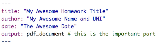
- Add PDF Dependencies: As stated when you create a new R Markdown file, the PDF output format requires TeX:
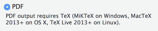
- Make sure you download TeX for your machine. Here are some Medium articles on the process of creating PDF reports (the articles cover starting from scratch with no installs at all, but you can skip over to installing TeX only):
This can be a little complicated, but it will make that Knit button near the top of the IDE magically generate a PDF for you.
If you are in a rush and want a shortcut, you can instead set the Default Output Format to HTML. When you open the file in your browser, you can save it as a PDF. It will not be as nicely formatted, but it will still work.
2.5 Getting help
 via
via First off…breeeeeeathe. We can fix this. There are a bunch of resources out there that can help you.
2.5.1 Things to try
Remember: Always try to help yourself! This article has a great list of tools to help you learn about anything you may be confused by. This includes learning about functions and packages as well as searching for info about a function/package/problem/etc. This is the perfect place to learn how to get the info you need.
The RStudio Help menu (in the top toolbar) is a fantastic place to go for understanding/fixing any problems. There are links to documentation and manuals as well as cheatsheets and a lovely collection of keyboard shortcuts.
Vignettes are a great way to learn about packages and how they work. Vignettes are like stylized manuals that can do a better job at explaining a package’s contents. For example,
ggplot2has a vignette on aesthetics calledggplot2-specsthat talks about different ways you can map data to different formats.- Typing
browseVignettes()in the console will show you all the vignettes for all of the packages you have installed. - You can also see vignettes by package by typing
vignette(package = "<package_name>")into the console. - To run a specific vignette, use
vignette("<vignette_name>"). If the vignette can’t be resolved, include the package name as well:vignette("<vignette_name", package = "<package_name>")
- Typing
Don’t ignore errors. They are telling you so much! If you give up because red text showed up in your console, take the time to see what that red text is saying. Learn how to read errors and what they are telling you. They usually include where the problem happened and what R thinks the problem stems from.
More Advanced: Learn to love debugger mode. Debugging can have a steep learning curve, but huge payoffs. Take a look at these videos about debugging with R. Topics include running the debugger, setting breakpoints, customizing preferences, and more. Note: R Markdown files have some limitations for debugging, as discussed in this article. You could also consider working out your code in a .R file before including it in your R Markdown homework submission.
2.5.2 Help me, R community!
Relax. There are a bunch of people using the same tools you are.
Your fellow classmates are a good place to start! Post questions to Piazza asking for help.
There is a lot of great documentation on R and its functions/packages/etc. Get comfy with R Documentation and it will help you immensely.
There is a vibrant RStudio Community page. Also, R likes twitter. Check out #rstats or maybe let Hadley Wickham know about a wonky error message.
with