16 Chart: Heatmap

16.1 Overview
This section covers how to make heatmaps.
16.2 tl;dr
Enough with these simple examples! I want a complicated one!
Here’s a heatmap of occupational categories of sons and fathers in the US, UK, and Japan:
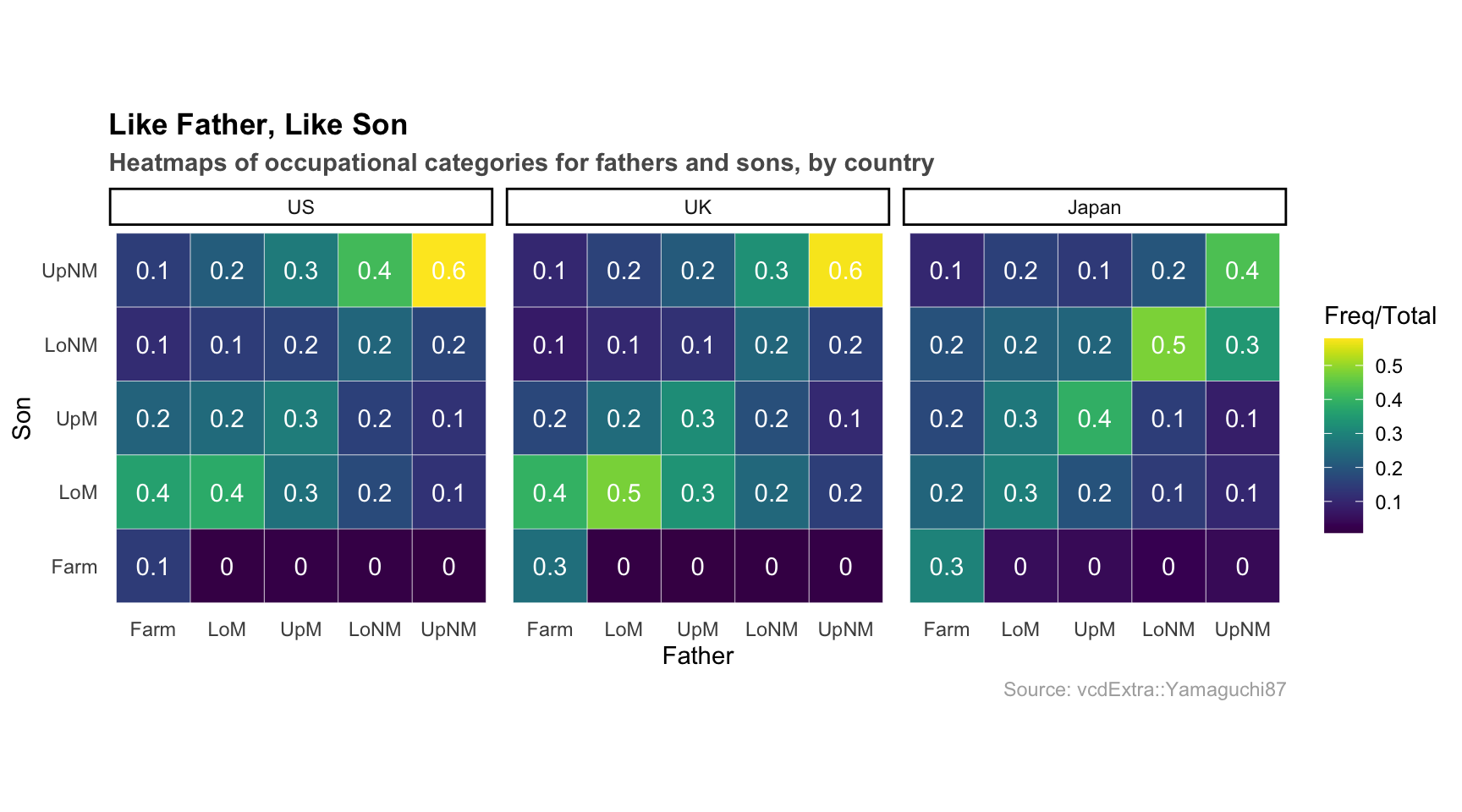
And here’s the code:
library(vcdExtra) # dataset
library(dplyr) # manipulation
library(ggplot2) # plotting
library(viridis) # color palette

# format data
orderedclasses <- c("Farm", "LoM", "UpM", "LoNM", "UpNM")
mydata <- Yamaguchi87
mydata$Son <- factor(mydata$Son, levels = orderedclasses)
mydata$Father <- factor(mydata$Father,
                        levels = orderedclasses)
japan <- mydata %>% filter(Country == "Japan")
uk <- mydata %>% filter(Country == "UK")
us <- mydata %>% filter(Country == "US")

# convert to % of country and class total
mydata_new <- mydata %>% group_by(Country, Father) %>%
  mutate(Total = sum(Freq)) %>% ungroup()

# make custom theme
theme_heat <- theme_classic() +
  theme(axis.line = element_blank(),
        axis.ticks = element_blank())

# basic plot
plot <- ggplot(mydata_new, aes(x = Father, y = Son)) +
  geom_tile(aes(fill = Freq/Total), color = "white") +
  coord_fixed() + facet_wrap(~Country) + theme_heat

# plot with text overlay and viridis color palette
plot + geom_text(aes(label = round(Freq/Total, 1)),
                 color = "white") +
      scale_fill_viridis() +
      # formatting
      ggtitle("Like Father, Like Son",
              subtitle = "Heatmaps of occupational categories for fathers and sons, by country") +
      labs(caption = "Source: vcdExtra::Yamaguchi87") +
      theme(plot.title = element_text(face = "bold")) +
      theme(plot.subtitle = element_text(face = "bold", color = "grey35")) +
      theme(plot.caption = element_text(color = "grey68"))
For more info on this dataset, type ?vcdExtra::Yamaguchi87 into the console.
16.3 Simple examples
Too complicated! Simplify, man!
16.3.1 Heatmap of two-dimensional bin counts
For this heatmap, we will use the SpeedSki dataset.
Only two variables, x and y are needed for two-dimensional bin count heatmaps. The third variable–i.e., the color–represents the bin count of points in the region it covers. Think of it as a two-dimensional histogram.
To create a heatmap, simply substitute geom_point() with geom_bin2d():
library(ggplot2) # plotting
library(GDAdata) # data (SpeedSki)

ggplot(SpeedSki, aes(Year, Speed)) +
  geom_bin2d()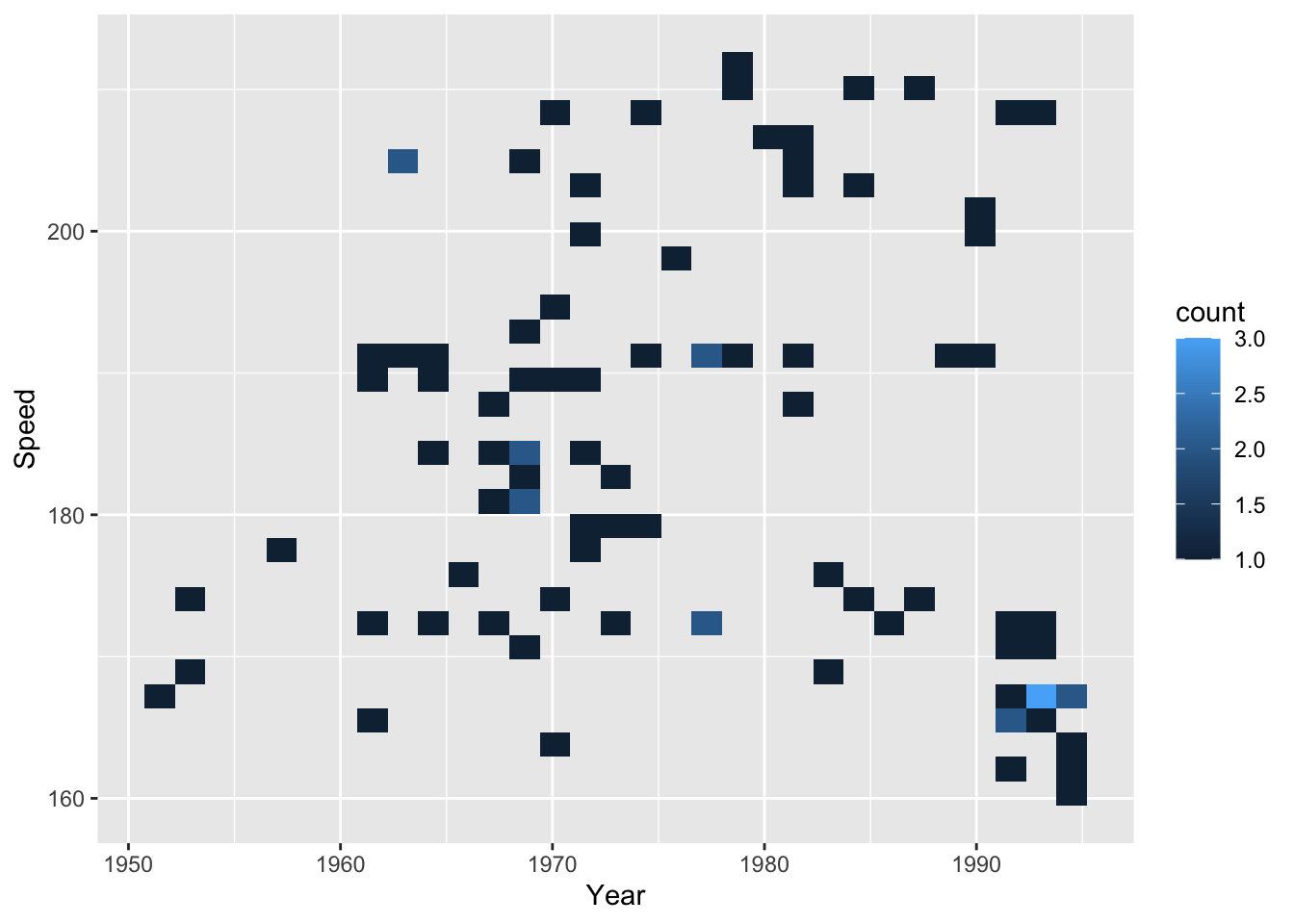
16.3.2 Heat map of dataframe
To get a visual sense of the dataframe, you can use a heatmap. You can also look into scaling the columns to get a sense of your data on a common scale. In this example, we use geom_tile to graph all cells in the dataframe and color them by their value:
library(pgmm) # data
library(tidyverse) # processing/graphing
library(viridis) # color palette

data(wine)

# convert to column, value
wine_new <- wine %>%
  rownames_to_column() %>%
  gather(colname, value, -rowname)

ggplot(wine_new, aes(x = rowname, y = colname, fill = value)) +
  geom_tile() + scale_fill_viridis() +
  ggtitle("Italian Wine Dataframe")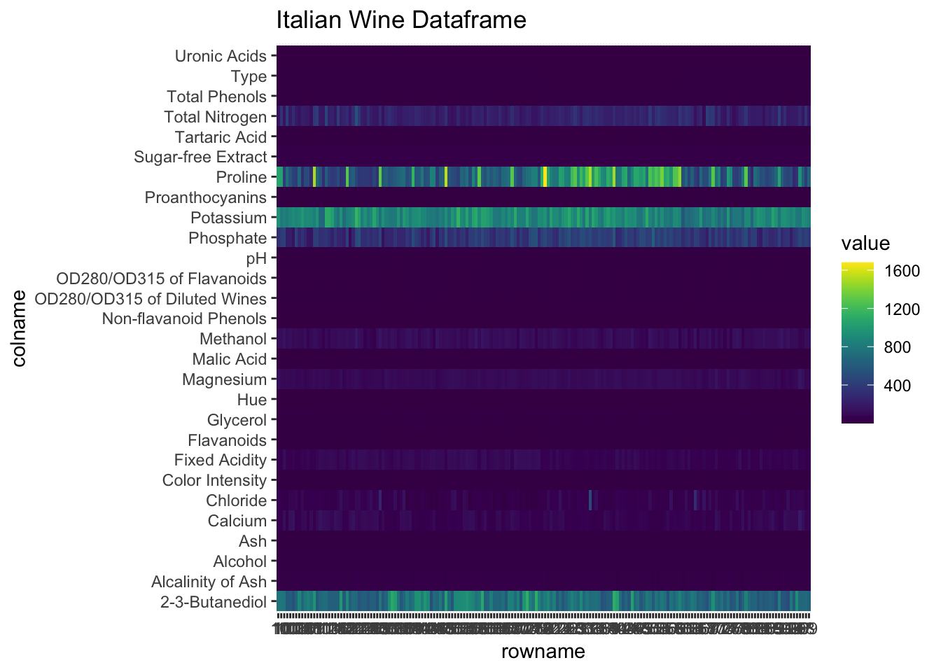
# only difference from above is scaling
wine_scaled <- data.frame(scale(wine)) %>%
  rownames_to_column() %>%
  gather(colname, value, -rowname)

ggplot(wine_scaled, aes(x = rowname, y = colname, fill = value)) +
  geom_tile() + scale_fill_viridis() +
  ggtitle("Italian Wine Dataframe, Scaled")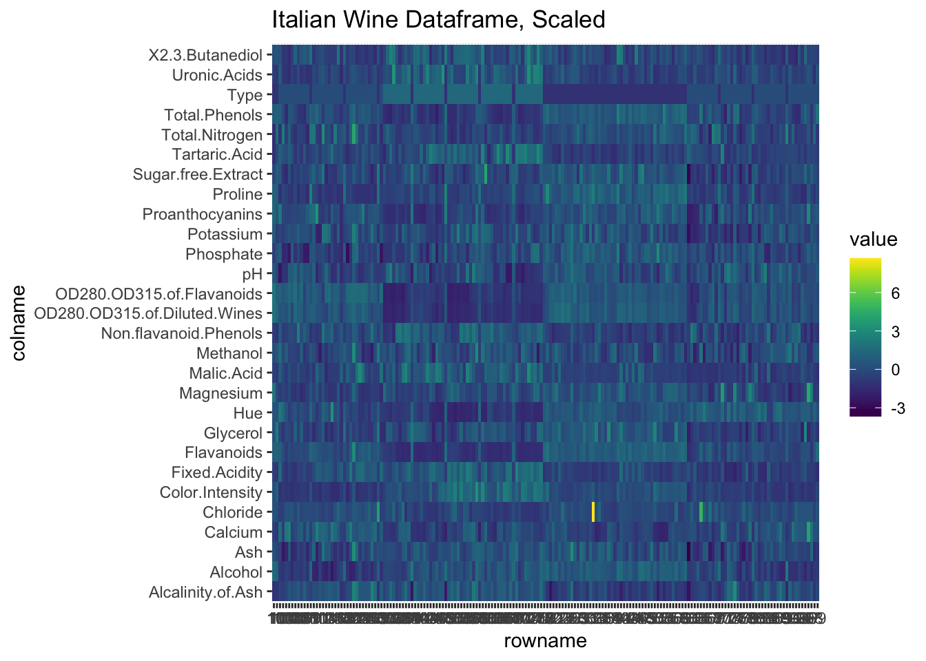
16.3.3 Modifications
You can change the color palette by specifying it explicitly in your chain of ggplot function calls. The bin width can be added inside the geom_bin2d() function call:
library(viridis) # viridis color palette

# create plot
g1 <- ggplot(SpeedSki, aes(Year, Speed)) +
  scale_fill_viridis() # modify color

# show plot
g1 + geom_bin2d(binwidth = c(5, 5)) # modify bin width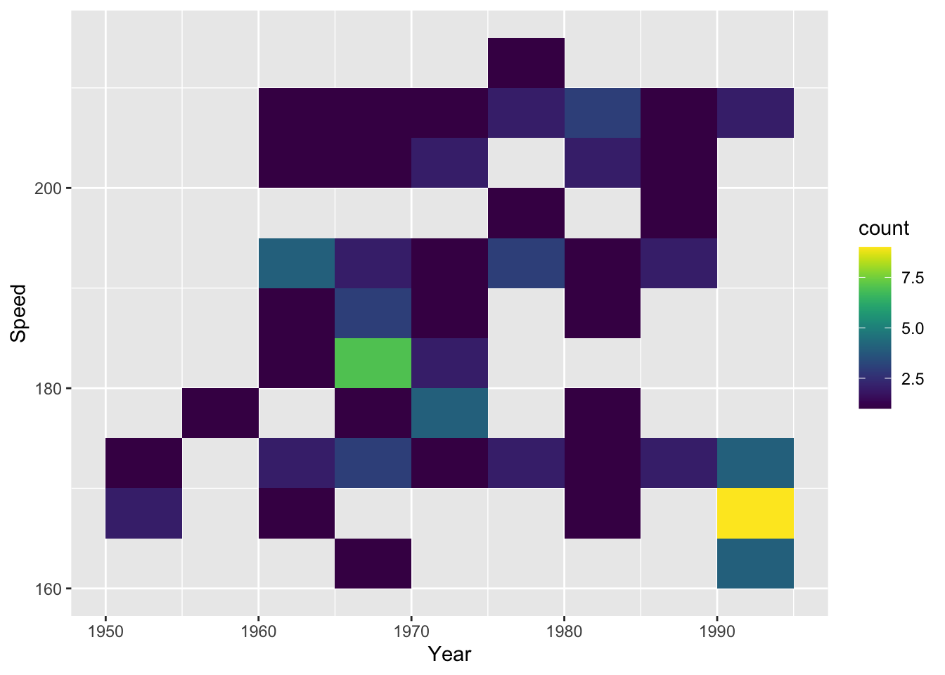
Here are some other examples:
# larger bin width
g1 + geom_bin2d(binwidth = c(10, 10)) 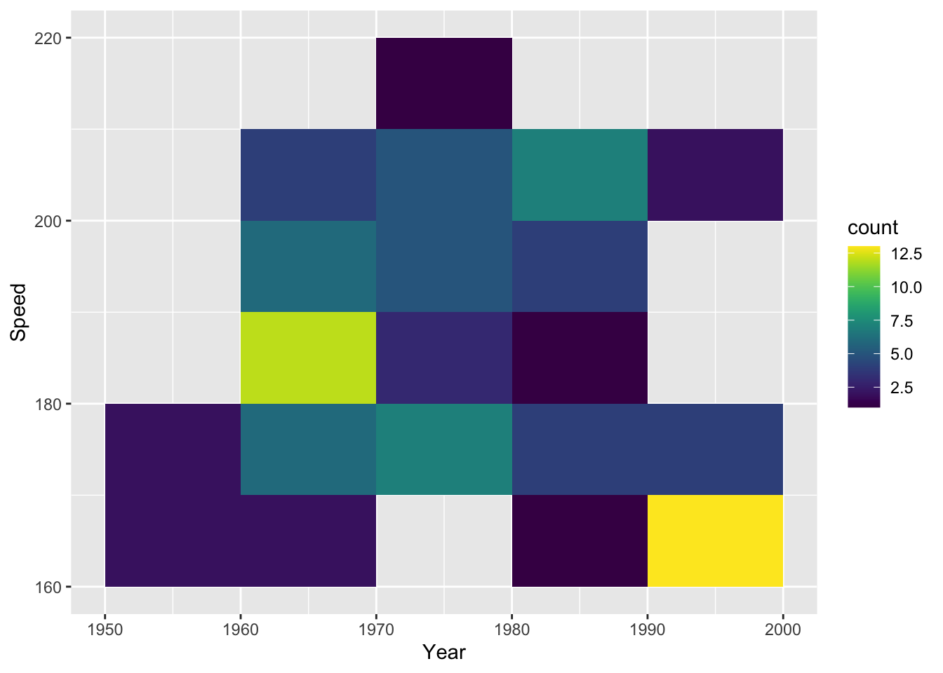
# hexagonal bins
g1 + geom_hex(binwidth = c(5, 5))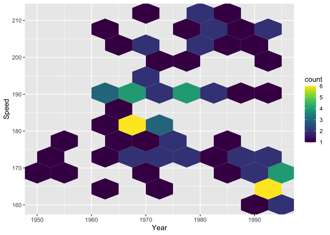
# hexagonal bins + scatterplot layer
g1 + geom_hex(binwidth = c(5, 5), alpha = .4) +
  geom_point(size = 2, alpha = 0.8)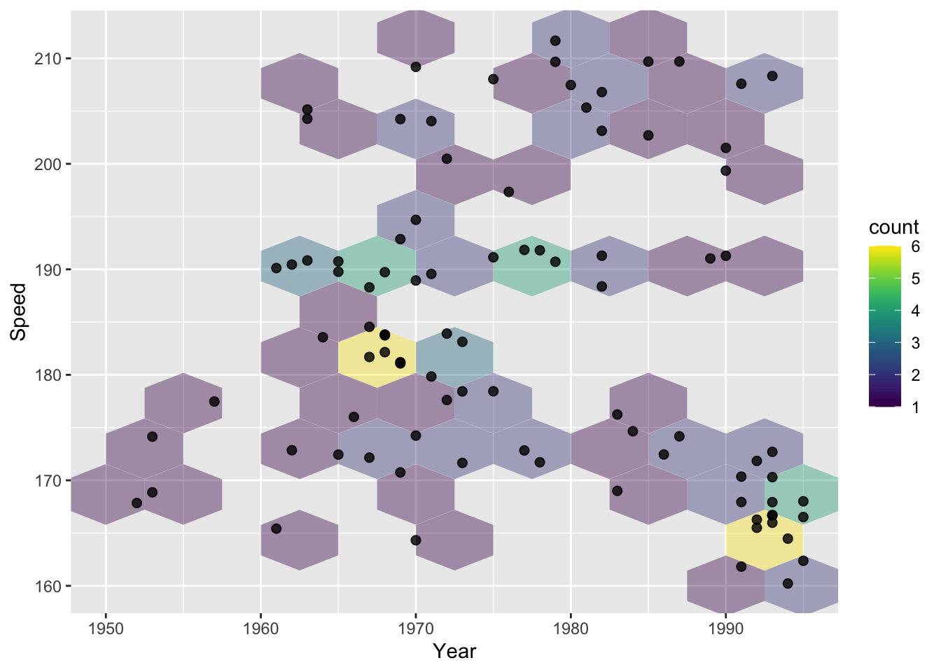
# hexagonal bins with custom color gradient/bin count
ggplot(SpeedSki, aes(Year, Speed)) +
  scale_fill_gradient(low = "#cccccc", high = "#09005F") + # color
  geom_hex(bins = 10) # number of bins horizontally/vertically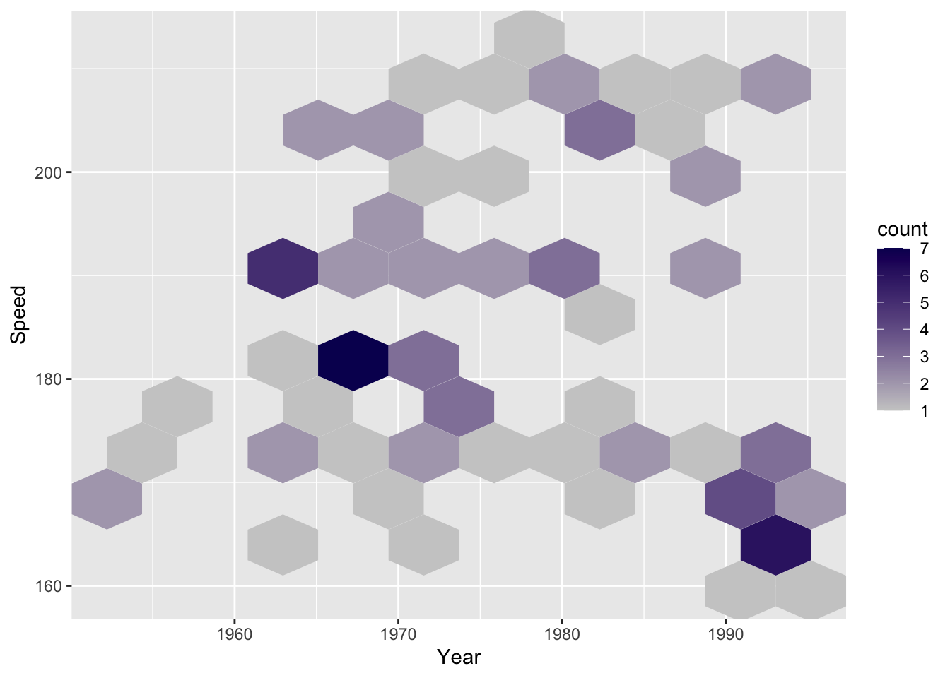
16.4 Theory
Heat maps are like a combination of scatterplots and histograms: they allow you to compare different parameters while also seeing their relative distributions.
- While heatmaps are visually striking, there are often better choices to get your point across. For more info, checkout this DataCamp section on heatmaps and alternatives.
16.5 External resources
- R Graph Gallery: Heatmaps: Has examples of creating heatmaps with the
heatmap()function. - How to make a simple heatmap in ggplot2: Create a heatmap with
geom_tile().
with