17 Spatial Data

This chapter is under active development. Check back soon for updates.

There are an overwhelming number of R packages for analyzing and visualizing spatial data. In broad terms, spatial visualizations require a merging of non-spatial and spatial information. For example, if you wish to create a choropleth map of the murder rate by county in New York State, you need county level data on murder rates, and you also need geographic data for drawing the county boundaries, stored in what are called shape files. A rough divide exists between packages that don’t require you deal with shape files and those that do. The former work by taking care of the geographic data under the hood: you supply the data with a column for the location and the package takes care of figuring out how to draw those locations. Not surprisingly, there are more easy-to-use options for commonly drawn maps, such as world continents, U.S. states, etc.

17.1 High level packages

17.1.1 Choropleth maps

Choropleth maps use color to indicate the value of a variable within a defined region, generally political boundaries. In this section we provide options that do not require you to work with shape files.

“Mapping in R” by Hanjun Li and Chengchao Jin explain how to use the maps package to create choropleth maps both with base R graphics and ggplot2. The maps package is U.S.-centered but also contains spatial data on a few other locations, as documented in the package reference manual. The choroplethr package makes it simple to draw choropleth maps of U.S. states, countries, and census tracts, as well as countries of the world without dealing directly with shape files. The companion package, choroplethrZip, provides data for zip code level choropleths; choroplethrAdmin1 draws choropleths for administrative regions of world countries. The following is a brief tutorial on using these packages.

Note: You must install also install choroplethrMaps for choroplethr to work. In addition, choroplethr requires a number of other dependencies which should be installed automatically, but if they aren’t, you can manually install the missing packages that you are notified about when you call library(choroplethr): maptools, and rgdal, sp.

We’ll use the state.x77 dataset for this example:

library(tidyverse)
library(choroplethr)

# data frame must contain "region" and "value" columns

df_illiteracy <- state.x77 %>% as.data.frame() %>% 
  rownames_to_column("state") %>% 
  transmute(region = tolower(`state`), value = Illiteracy)

state_choropleth(df_illiteracy,
                 title = "State Illiteracy Rates, 1977",
                 legend = "Percent Illiterate")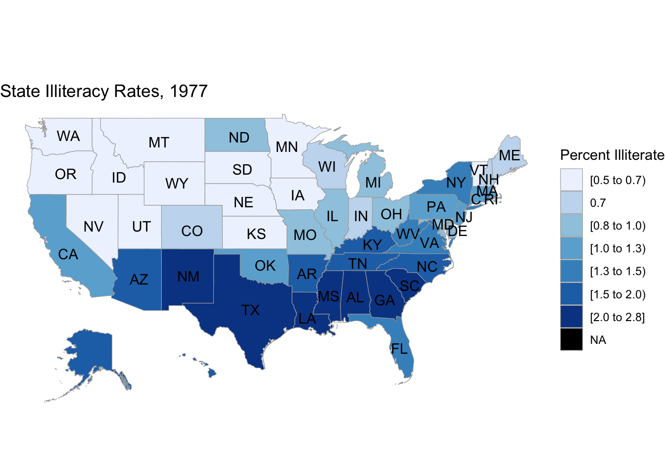

17.1.2 Square bins

Packages such as statebins create choropleth style maps with equal size regions that roughly represent the location of the region, but not the size or shape.

Important: Don’t install statebins from CRAN; use the dev version – it contains many improvements, which are detailed in “Statebins Reimagined”.

# devtools::install_github("hrbrmstr/statebins")
library(statebins)
df_illit <- state.x77 %>% as.data.frame() %>% 
  rownames_to_column("state") %>% 
  select(state, Illiteracy)

# Note: direction = 1 switches the order of the fill scale 
# so darker shades represent higher illiteracy rates
# (The default is -1).

statebins(df_illit, value_col="Illiteracy",
          name = "%", direction = 1) +
  ggtitle("State Illiteracy Rates, 1977") +
  theme_statebins()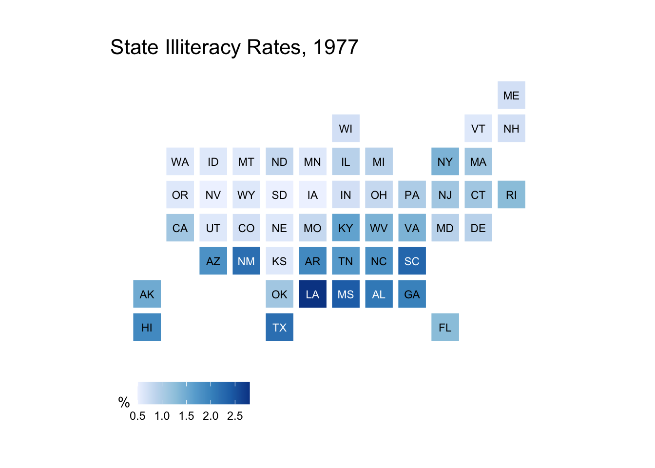

17.1.3 Longitude / latitude data

Note that the options above work with political boundaries, based on the names of the regions that you provide. Such maps require packages with geographical boundary information. Longitude / latitude data, on the other hand, can be plotted simply as a scatterplot with x = longitude and y = latitude, without any background maps (just don’t mix up x & y!) The first part of “Data wrangling visualisation and spatial analysis: R Workshop” by C. Brown, D. Schoeman, A. Richardson, and B. Venables provides a detailed walkthrough of spatial exploratory data analysis with copepod data (a type of zooplankton) using this technique with ggplot2::geom_point(). It is a highly recommended resource as it covers much of the data science pipeline from the context of the problem to obtaining data, cleaning and transforming it, exploring the data, and finally modeling and predicting.

Adding a background map to lon/lat data requires pulling a map from a map API and setting a bounding box. This can be done easily with ggmap, which offers several different map source options. Google Maps API was the go-to, but they now require you to enable billing through Google Cloud Platorm. You get $300 in free credit, but if providing a credit card isn’t your thing, you may consider using Stamen Maps instead, with the get_stamenmap() function. Use the development version of the package; instructions and extensive examples are available on the package’s GitHub page “Stamen Maps with ggmap” by Mrugank Akarte offers an introductory tutorial. “Getting started Stamen maps with ggmap” will help you get started with Stamen maps through an example using the Sacramento dataset in the caret package.

17.2 Shape files and more

“Plotting Maps with R: An Example-Based Tutorial” by Jonathan Santoso and Kevin Wibisono provides an introduction to working with shape files using the rgdal package and plotting maps with base R graphics, ggmap, leaflet, and tmap.

“Mapping in R just got a whole lot easier” by Sharon Machlis (2017-03-03) offers a tutorial on using the tmap, tmaptools, and tigris packages to create choropleth maps. Note that with this approach, you will need to merge geographic shape files with your data files, and then map.

“Step-by-Step Choropleth Map in R: A case of mapping Nepal” walks through the process of creating a choropleth map using rgdal and ggplot2.

The second part of the copepod data tutorial of the mentioned above provides examples using the maps and sf packages. You’ll learn how to set bounding boxes and change the map projection. The tutorial concludes with an interactive map created with leaflet.

17.3 State-of-the-art

If you’re serious about learning how to create maps in R, Geocomputation in R by Robin Lovelace, Jakub Nowosad, and Jannes Muenchow is the place to start. This book focuses on the tmap package, but is much more than a technical how-to, providing a theoretical context for working with geographical data.

with