24 Outliers
 This chapter originated as a community contribution created by kiransaini
This page is a work in progress. We appreciate any input you may have. If you would like to help improve this page, consider contributing to our repo.
24.1 Overview
This section covers what types of outliers are encountered in data and how to handle them.
24.2 tl;dr
I want to see my outliers!
Outliers are difficult to spot because judging a datapoint as an outlier depends on the data or model with which they are compared. It is important to detect outliers because they can distort predictions and affect the accuracy of the model.
24.3 What are outliers?
Outliers are noticeably far from the bulk of the data. They can be errors, genuine extreme values, rare values, unusual values, cases of special interest, or data from another source. Outliers on individual variables can be spotted using boxplots and bivariate outliers can be spotted using scatterplots. There can also be higher dimensional outliers that are not outliers in lower dimensions.
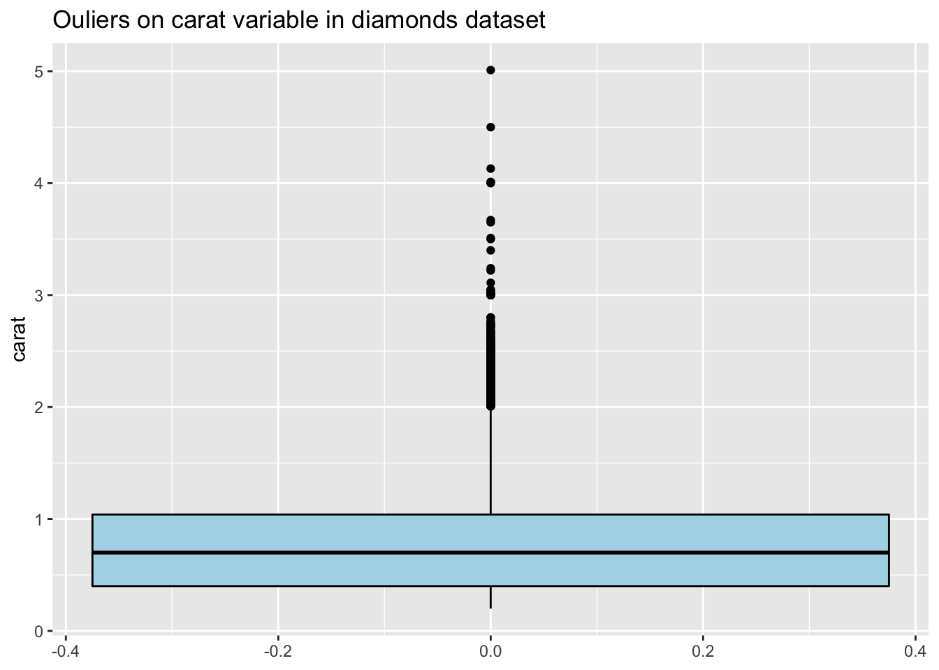
It is worth identifying outliers for a number of reasons. Bad outliers should always be corrected and many statistical methods may work poorly in presence of outliers, but genuine outlying values can be interesting in their own right. Let’s have a look at the outliers of the ‘carat’ variable in the diamonds dataset:
24.4 Types of Outliers
24.4.1 Univariate Outliers
Univariate outliers are outlying along one dimension. The best-known approach for an initial look at the data is to use boxplots. Tukey suggests marking individual cases as outliers if they are more than 1.5 IQR (the interquartile range) outside the hinges (basically the quartiles). Outliers may change if they are grouped by another variable. Let’s have a look at outliers on the Sepal Width variable in the iris dataset, both when the data is grouped by Species and when it is not. The outliers are clearly different:
p <- ggplot(iris, aes(x=Species, y=Sepal.Width)) +
  geom_boxplot(color="black", fill="lightblue") +
  ggtitle("Boxplot for Sepal Width grouped by Species in iris dataset")
p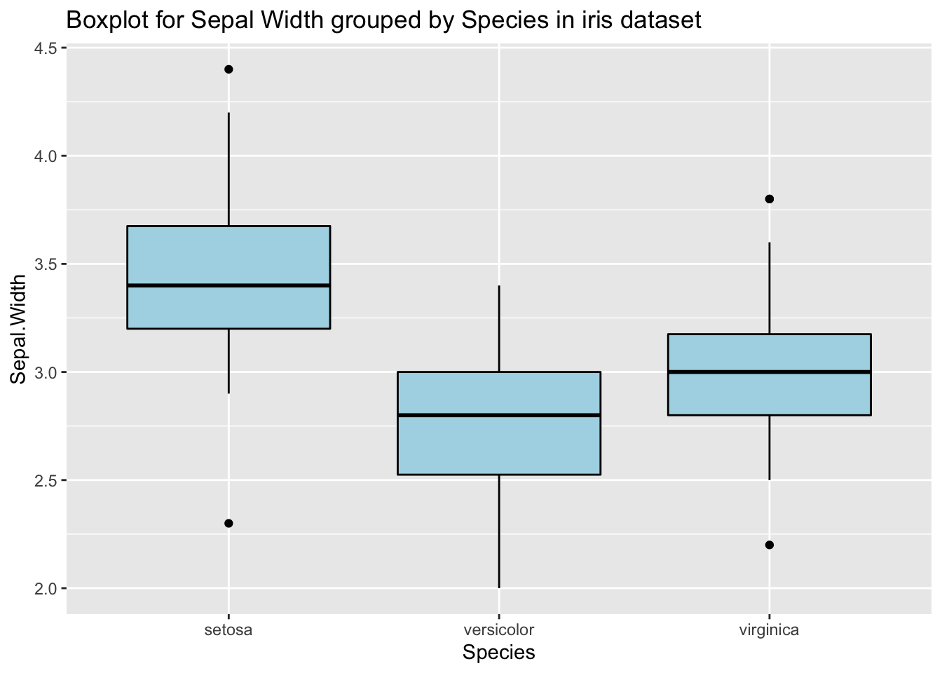
p <- ggplot(iris, aes(y=Sepal.Width)) +
  geom_boxplot(color="black", fill="lightblue") +
  ggtitle("Boxplot for Sepal Width in iris dataset")
p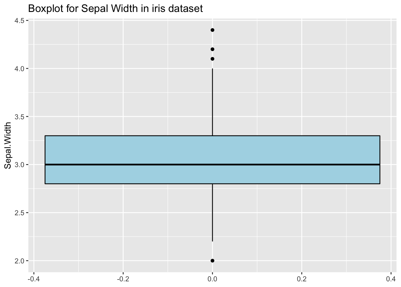
24.4.2 Multivariate Outliers
Multivariate outliers are outlying along more than one dimension. Scatterplots and parallel coordinate plots are useful for visualizing multivariate outliers. You could regard points as outliers that are far from the mass of the data, or you could regard points as outliers that do not fit the smooth model well. Some points are outliers on both criteria. Let’s have a look at outliers on the Petal Length and Sepal Width variables in the iris dataset. We can clearly see an outlier which is far from the mass of the data (lower left):
ggplot(iris, aes(x=Sepal.Width, y=Petal.Length)) +
  geom_point() +
  ggtitle("Scatterplot for Petal Length vs Sepal Width in iris dataset")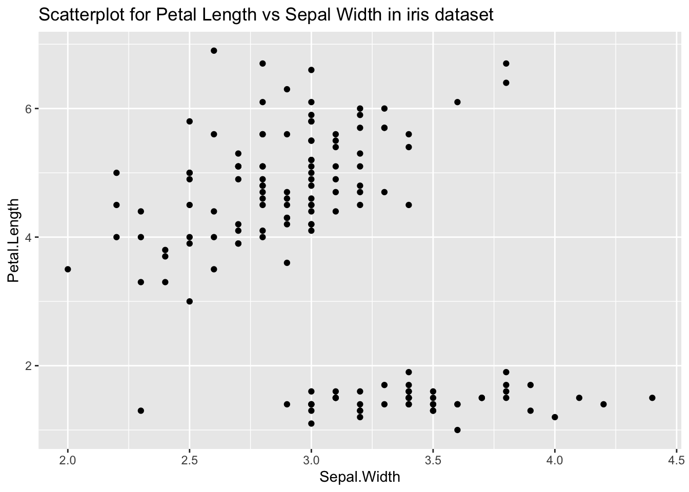
Let’s have a look at outliers on the Petal Length and Petal Width variables in the iris dataset by fitting a smooth model. Here the outliers are the points that do not fit the smooth model:
ggplot(iris, aes(x=Petal.Width, y=Petal.Length)) +
  geom_point() +
  geom_smooth() +
  geom_density2d(col="red",bins=4) +
  ggtitle("Scatterplot for Petal Length vs Petal Width in iris dataset")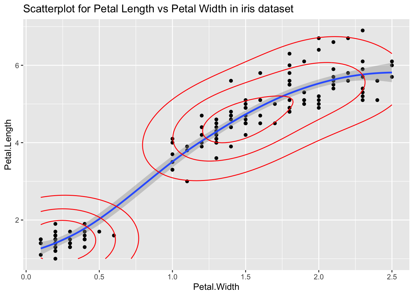
Lets have a look at outliers in the diamond dataset using a parallel coordinate plot. We can see an outlier on the carat, cut, color, and clarity variables that is not an outlier on individual variables:
library(GGally)
ggparcoord(diamonds[1:1000,], columns=1:5, scale="uniminmax", alpha=0.8) +
  ggtitle("Parallel coordinate plot of diamonds dataset")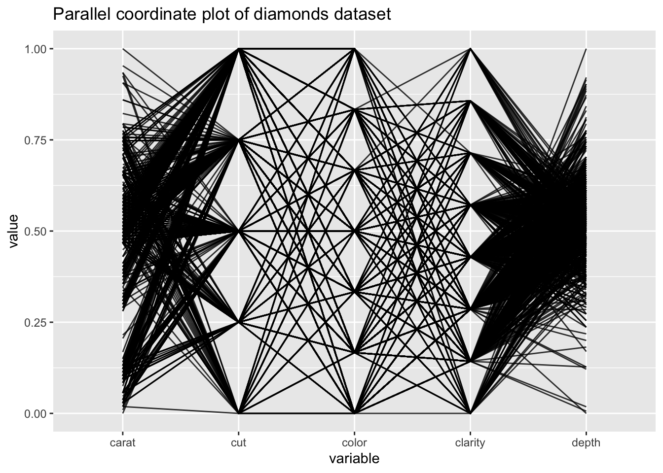
24.4.3 Categorical Outliers
Outliers can be rare on a categorical scale. Certain combinations of categories are rare or should not occur at all. Fluctuation diagrams can be used to find such outliers. We can see rare cases in the HairEyeColor dataset:
library(datasets)
#fluctile(HairEyeColor) from extracat package, no longer on CRAN
24.5 Handling Outliers
Identifying outliers using plots and fitting models is relatively easy compared to what to do after identifying the outliers. Outliers can be rare cases, unusual values, or genuine errors. Genuine errors must be corrected if possible or else they must be removed. Imputation of outliers is complicated and appropriate background knowledge is required.
A strategy for dealing with outliers is as follows
Plot the one-dimensional distributions of the variables using boxplots. Examine any extreme outliers to see if they are rare values or errors and decide if they should be removed or imputed.
For outliers which are extreme on one dimension, examine their values on other dimensions to decide whether they should be discarded or not. Discard values that are outliers on more than one dimension.
Consider cases which are outliers in a higher dimensions but not in lower dimensions. Decide whether they are errors or not and consider discarding or imputing the errors.
Plot boxplots and parallel coordinate plots by using grouping on a variable to find outliers in subsets of the data.
24.5.1 Not informative
Consider the diamonds dataset. Let’s have a look at the width (y) and depth (z) variables:
ggplot(diamonds, aes(y=y)) +
  geom_boxplot(color="black", fill="#9B3535") +
  ggtitle("Ouliers on width variable in diamonds dataset")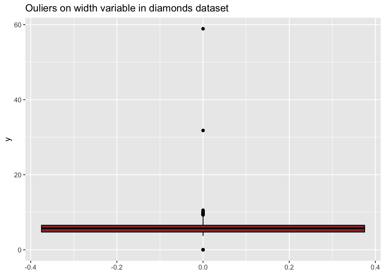
ggplot(diamonds, aes(y=z)) +
  geom_boxplot(color="black", fill="#9B3535") +
  ggtitle("Ouliers on depth variable in diamonds dataset")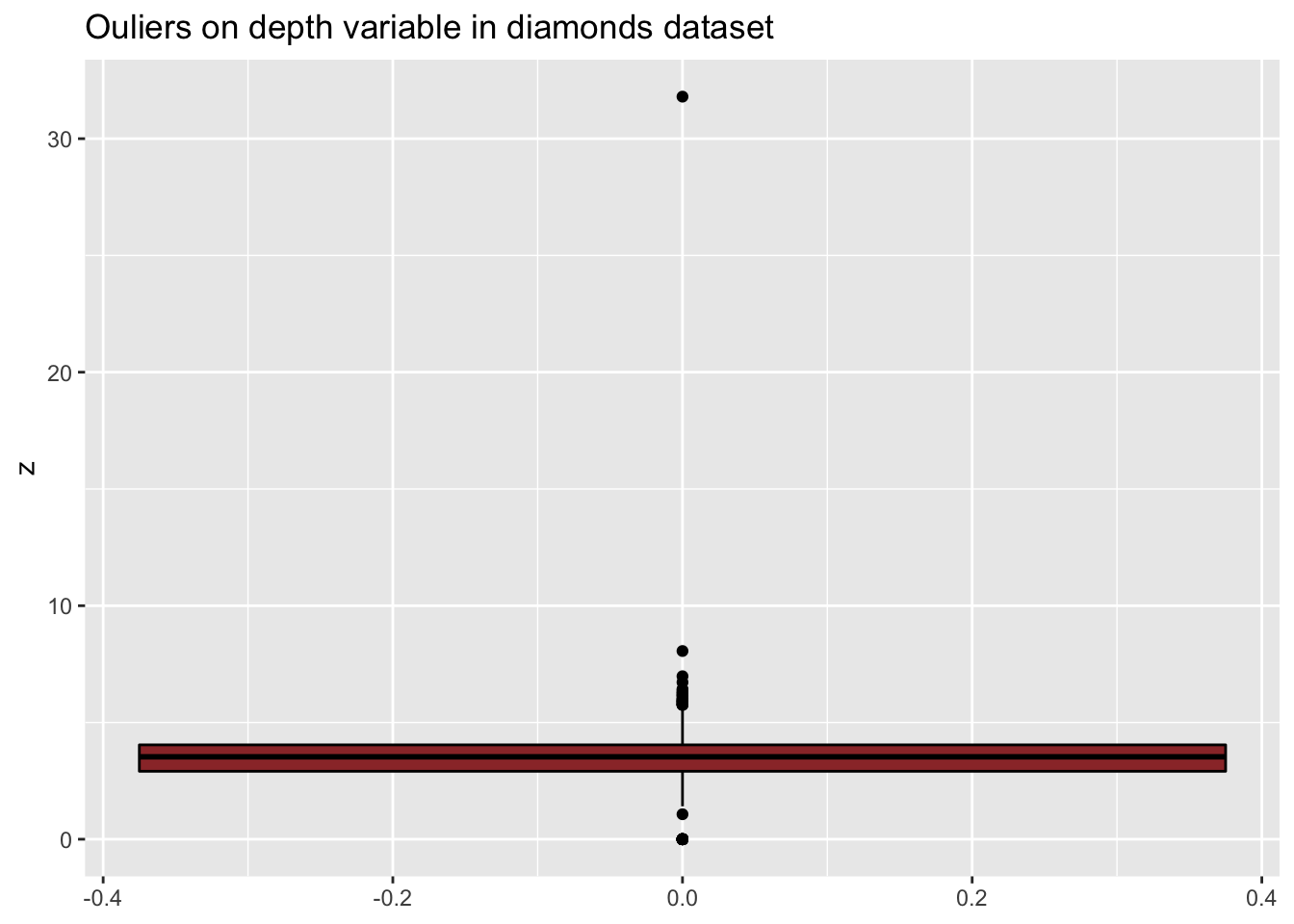
ggplot(diamonds, aes(y, z)) +
  geom_point(col = "#9B3535") +
  xlab("width") +
  ylab("depth")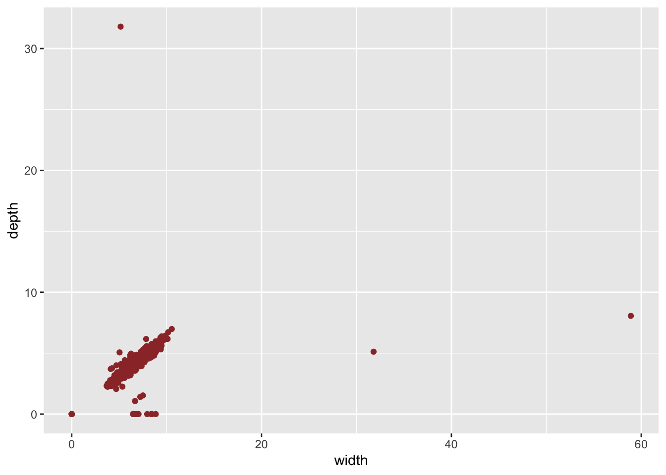
24.5.2 More informative
The plots are not very informative due to the outliers. The same plots after filtering the outliers are much more informative:
d2 <- filter(diamonds, y > 2 & y < 11 & z > 1 & z < 8)
ggplot(d2, aes(y=y)) +
  geom_boxplot(color="black", fill="lightblue") +
  ggtitle("Ouliers on width variable in diamonds dataset")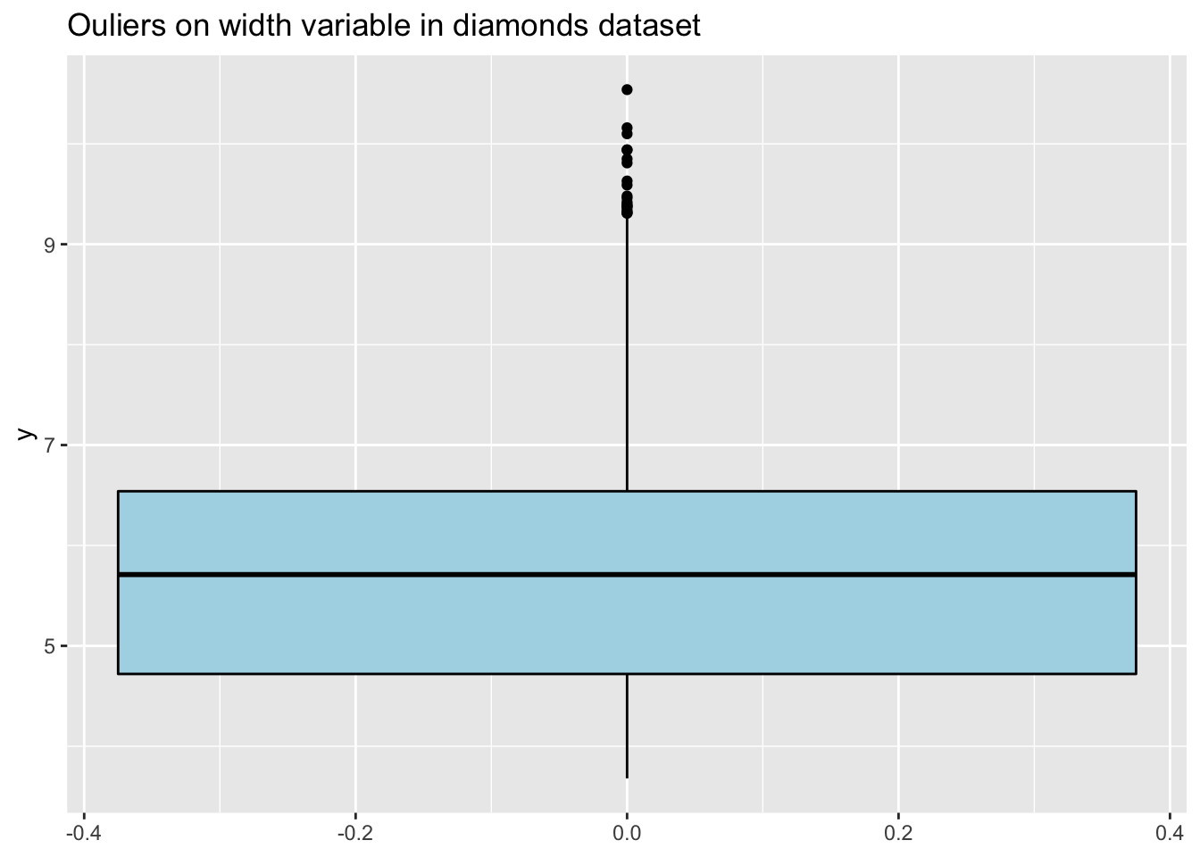
d2 <- filter(diamonds, y > 2 & y < 11 & z > 1 & z < 8)
ggplot(d2, aes(y=z)) +
  geom_boxplot(color="black", fill="lightblue") +
  ggtitle("Ouliers on depth variable in diamonds dataset")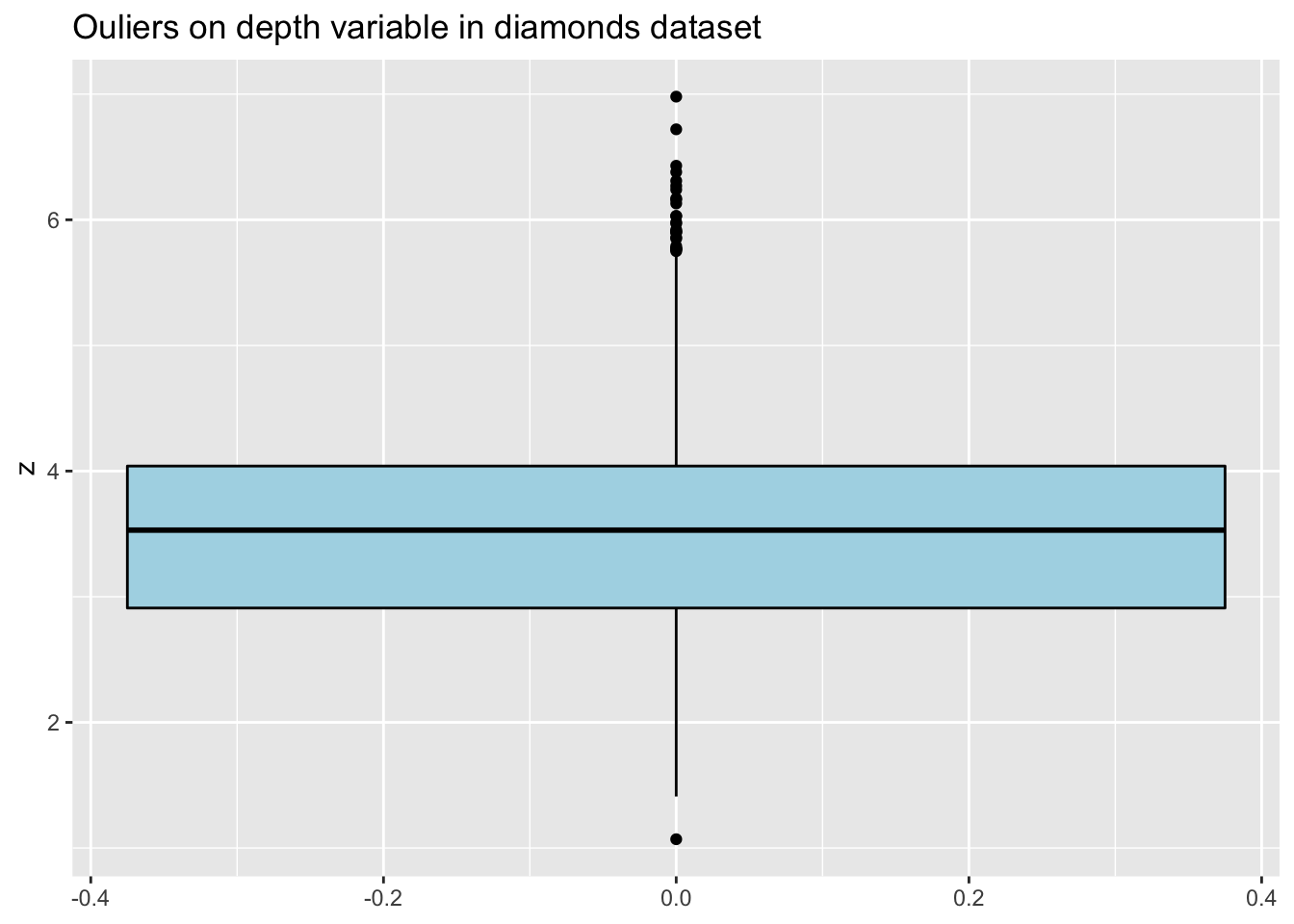
d2 <- filter(diamonds, y > 2 & y < 11 & z > 1 & z < 8)
ggplot(d2, aes(y, z)) +
  geom_point(shape = 21, color = "darkGrey", fill = "lightBlue", stroke = 0.1) +
  xlab("width") +
  ylab("depth")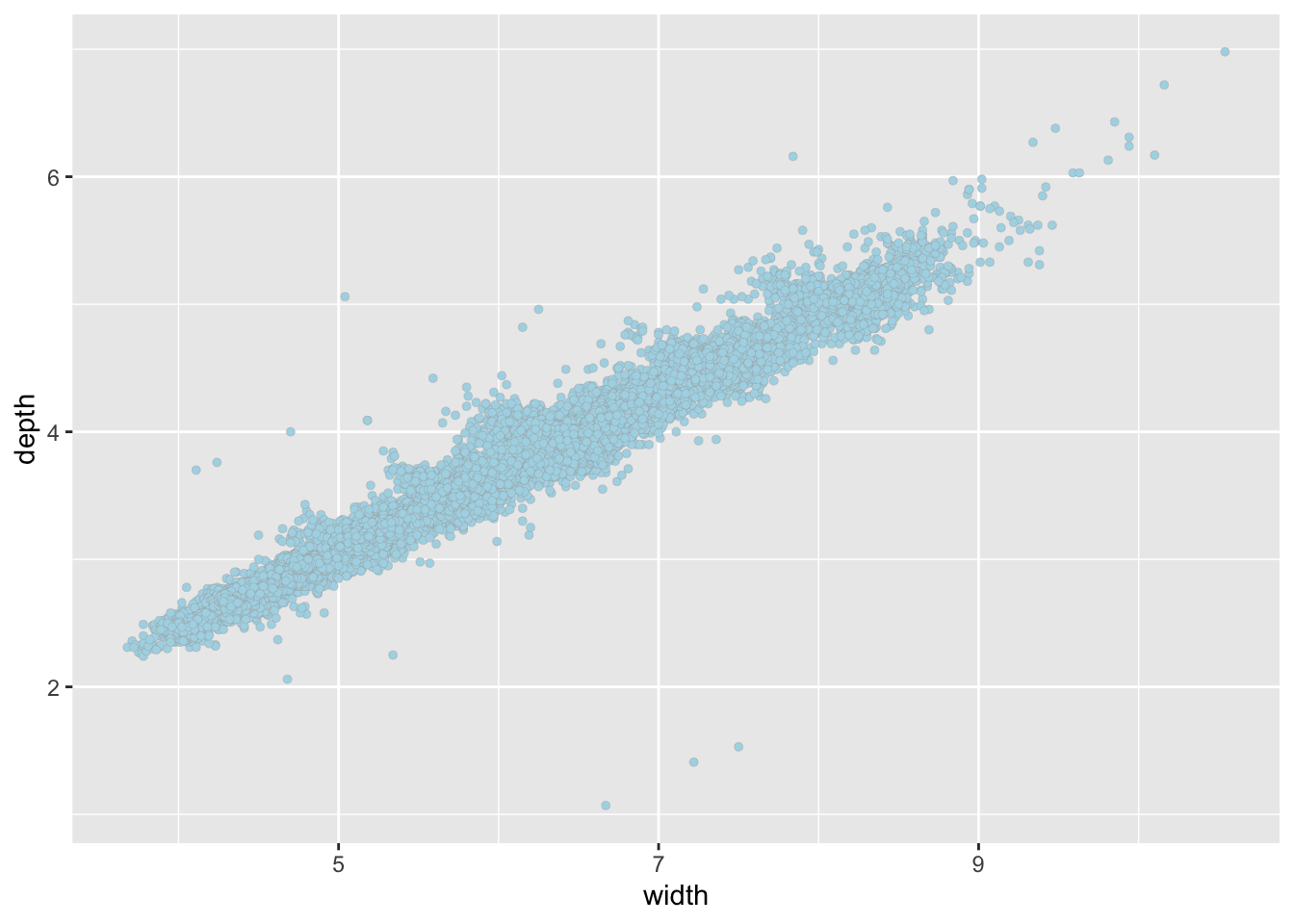
24.6 External Resources
Identify, describe, plot, and remove the outliers from the dataset: Plotting and removing outliers from a dataset
A Brief Overview of Outlier Detection Techniques: Discussion of the theoretical aspect of outlier detection
with