22 Walkthrough: Tidy Data & dplyr
 This chapter originated as a community contribution created by akshatapatel
This page is a work in progress. We appreciate any input you may have. If you would like to help improve this page, consider contributing to our repo.
22.1 Overview
This example goes through some work with the biopsy dataset using dplyr functions to get to a tidy dataset.
22.2 Installing packages
Write the following statements in the console:
install.packages('dplyr')install.packages('ggplot2')install.packages('tidyr')install.packages('MASS')
Note: The first three packages are a part of the tidyverse, a collection of helpful packages in R, which can all be installed using install.packages('tidyverse').
dplyr is used for data wrangling and data transformation in data frames. The “d” in “dplyr” stands for “data frames” which is the most-used data type for storing datasets in R.
22.3 Viewing the data
Let’s start with loading the package so we can get the data as a dataframe:
#loading the dplyr library
library(dplyr)

#loading data from MASS:biopsy
data(biopsy, package = "MASS")
class(biopsy)
## [1] "data.frame"#glimpse is a part of the dplyr package
glimpse(biopsy)## Rows: 699
## Columns: 11
## $ ID <chr> "1000025", "1002945", "1015425", "1016277", "1017023", "1017122"…
## $ V1 <int> 5, 5, 3, 6, 4, 8, 1, 2, 2, 4, 1, 2, 5, 1, 8, 7, 4, 4, 10, 6, 7, …
## $ V2 <int> 1, 4, 1, 8, 1, 10, 1, 1, 1, 2, 1, 1, 3, 1, 7, 4, 1, 1, 7, 1, 3, …
## $ V3 <int> 1, 4, 1, 8, 1, 10, 1, 2, 1, 1, 1, 1, 3, 1, 5, 6, 1, 1, 7, 1, 2, …
## $ V4 <int> 1, 5, 1, 1, 3, 8, 1, 1, 1, 1, 1, 1, 3, 1, 10, 4, 1, 1, 6, 1, 10,…
## $ V5 <int> 2, 7, 2, 3, 2, 7, 2, 2, 2, 2, 1, 2, 2, 2, 7, 6, 2, 2, 4, 2, 5, 6…
## $ V6 <int> 1, 10, 2, 4, 1, 10, 10, 1, 1, 1, 1, 1, 3, 3, 9, 1, 1, 1, 10, 1, …
## $ V7 <int> 3, 3, 3, 3, 3, 9, 3, 3, 1, 2, 3, 2, 4, 3, 5, 4, 2, 3, 4, 3, 5, 7…
## $ V8 <int> 1, 2, 1, 7, 1, 7, 1, 1, 1, 1, 1, 1, 4, 1, 5, 3, 1, 1, 1, 1, 4, 1…
## $ V9 <int> 1, 1, 1, 1, 1, 1, 1, 1, 5, 1, 1, 1, 1, 1, 4, 1, 1, 1, 2, 1, 4, 1…
## $ class <fct> benign, benign, benign, benign, benign, malignant, benign, benig…head(biopsy)## ID V1 V2 V3 V4 V5 V6 V7 V8 V9 class
## 1 1000025 5 1 1 1 2 1 3 1 1 benign
## 2 1002945 5 4 4 5 7 10 3 2 1 benign
## 3 1015425 3 1 1 1 2 2 3 1 1 benign
## 4 1016277 6 8 8 1 3 4 3 7 1 benign
## 5 1017023 4 1 1 3 2 1 3 1 1 benign
## 6 1017122 8 10 10 8 7 10 9 7 1 malignant22.4 What is Tidy data?
What does it mean for your data to be tidy?
Tidy data has a standardized format and it is a consistent way to organize your data in R.
Here’s the definition of Tidy Data given by Hadley Wickham:
A dataset is messy or tidy depending on how rows, columns and tables are matched up with observations, variables and types. In tidy data:
Each variable forms a column.
Each observation forms a row.
Each observational unit forms a value in the table.
See r4ds on tidy data for more info.
What are the advantages of tidy data?
Uniformity : It is easier to learn the tools that work with the data because they have a consistent way of storing data.
Most built-in R functions work with vectors of values. Thus, having variables as columns/vectors allows R’s vectorized nature to shine.
Can you observe and tell why this data is messy?
The names of the columns such as V1, V2 are not intuitive in what they contain; good sign it is untidy.
They are not different variables, but are values of a common variable.
Now, we will see the how to transform our data using dplyr functions and then look at how to tidy our transformed data.
22.5 Tibbles
A tibble is a modern re-imagining of the data frame.
It is particularly useful for large datasets because it only prints the first few rows. It helps you confront problems early, leading to cleaner code.
# Converting a df to a tibble
biopsy <- tbl_df(biopsy)
biopsy
## # A tibble: 699 × 11
## ID V1 V2 V3 V4 V5 V6 V7 V8 V9 class
## <chr> <int> <int> <int> <int> <int> <int> <int> <int> <int> <fct>
## 1 1000025 5 1 1 1 2 1 3 1 1 benign
## 2 1002945 5 4 4 5 7 10 3 2 1 benign
## 3 1015425 3 1 1 1 2 2 3 1 1 benign
## 4 1016277 6 8 8 1 3 4 3 7 1 benign
## 5 1017023 4 1 1 3 2 1 3 1 1 benign
## 6 1017122 8 10 10 8 7 10 9 7 1 malignant
## 7 1018099 1 1 1 1 2 10 3 1 1 benign
## 8 1018561 2 1 2 1 2 1 3 1 1 benign
## 9 1033078 2 1 1 1 2 1 1 1 5 benign
## 10 1033078 4 2 1 1 2 1 2 1 1 benign
## # … with 689 more rows22.6 Test for missing values
# Number of missing values in each column in the data frame
colSums(is.na(biopsy))
## ID V1 V2 V3 V4 V5 V6 V7 V8 V9 class
## 0 0 0 0 0 0 16 0 0 0 0The dataset contains missing values which need to be addressed.
22.7 Recode the missing values
One way to deal with missing values is to recode them with the average of all the other values in that column:
#change all the NAs to mean of the column
biopsy$V6[is.na(biopsy$V6)] <- mean(biopsy$V6, na.rm = TRUE)
colSums(is.na(biopsy))
## ID V1 V2 V3 V4 V5 V6 V7 V8 V9 class
## 0 0 0 0 0 0 0 0 0 0 0See our chapter on time series with missing data for more info about dealing with missing data.
22.8 Data wrangling verbs
Here are the most commonly used functions that help wrangle and summarize data:
- Rename
- Select
- Mutate
- Filter
- Arrange
- Summarize
- Group_by
Select and mutate functions manipulate the variable (the columns of the data frame). Filter and arrange functions manipulate the observations (the rows of the data) ,whereas the summarize function manipulates groups of observations.
All the dplyr functions work on a copy of the data and return a modified copy. They do not change the original data frame. If we want to access the results afterwards, we need to save the modified copy.
22.9 Rename
The names of the columns in our biopsy data are very vague and do not give us the meaning of the values in that column. We need to change the names of the column so that the viewer gets a sense of the values they’re referring to.
rename(biopsy,
       thickness = V1,cell_size = V2,
       cell_shape = V3, marg_adhesion = V4,
       epithelial_cell_size = V5, bare_nuclei = V6,
       chromatin = V7, norm_nucleoli = V8, mitoses = V9)
## # A tibble: 699 × 11
## ID thickness cell_size cell_shape marg_adhesion epithelial_cell_size
## <chr> <int> <int> <int> <int> <int>
## 1 1000025 5 1 1 1 2
## 2 1002945 5 4 4 5 7
## 3 1015425 3 1 1 1 2
## 4 1016277 6 8 8 1 3
## 5 1017023 4 1 1 3 2
## 6 1017122 8 10 10 8 7
## 7 1018099 1 1 1 1 2
## 8 1018561 2 1 2 1 2
## 9 1033078 2 1 1 1 2
## 10 1033078 4 2 1 1 2
## # … with 689 more rows, and 5 more variables: bare_nuclei <dbl>,
## # chromatin <int>, norm_nucleoli <int>, mitoses <int>, class <fct>The tibble shown above is not saved and cannot be used further. To use it afterwards we save it as a new tibble:
#saving the rename function output
biopsy_new<-rename(biopsy,
       thickness = V1,cell_size = V2,
       cell_shape = V3, marg_adhesion = V4,
       epithelial_cell_size = V5, bare_nuclei = V6,
       chromatin = V7, norm_nucleoli = V8, mitoses = V9)

head(biopsy_new,5)
## # A tibble: 5 × 11
## ID thickness cell_size cell_shape marg_adhesion epithelial_cell_size
## <chr> <int> <int> <int> <int> <int>
## 1 1000025 5 1 1 1 2
## 2 1002945 5 4 4 5 7
## 3 1015425 3 1 1 1 2
## 4 1016277 6 8 8 1 3
## 5 1017023 4 1 1 3 2
## # … with 5 more variables: bare_nuclei <dbl>, chromatin <int>,
## # norm_nucleoli <int>, mitoses <int>, class <fct>The biopsy_new data frame can now be used for further manipulation.
22.10 Select
Select returns a subset of the data. Specifically, only the columns that are specified are included.
In the biopsy data, we do not require the variables “chromatin” and “mitoses”. So, let’s drop them using a minus sign:
#selecting all except the columns chromatin and mitoses
biopsy_new<-select(biopsy_new,-chromatin,-mitoses)

head(biopsy_new,5)
## # A tibble: 5 × 9
## ID thickness cell_size cell_shape marg_adhesion epithelial_cell_size
## <chr> <int> <int> <int> <int> <int>
## 1 1000025 5 1 1 1 2
## 2 1002945 5 4 4 5 7
## 3 1015425 3 1 1 1 2
## 4 1016277 6 8 8 1 3
## 5 1017023 4 1 1 3 2
## # … with 3 more variables: bare_nuclei <dbl>, norm_nucleoli <int>, class <fct>22.11 Mutate
The mutate function computes new variables from the already existing variables and adds them to the dataset. It gives information that the data already contained but was never displayed.
The “V6” variable contains the values of the bare nucleus from 1.00 to 10.00. If we wish to normalize the variable, we can use the mutate function:
#normalize the bare nuclei values
maximum_bare_nuclei<-max(biopsy_new$bare_nuclei,na.rm=TRUE)
biopsy_new<-mutate(biopsy_new,bare_nuclei=bare_nuclei/maximum_bare_nuclei)

head(biopsy_new,5)
## # A tibble: 5 × 9
## ID thickness cell_size cell_shape marg_adhesion epithelial_cell_size
## <chr> <int> <int> <int> <int> <int>
## 1 1000025 5 1 1 1 2
## 2 1002945 5 4 4 5 7
## 3 1015425 3 1 1 1 2
## 4 1016277 6 8 8 1 3
## 5 1017023 4 1 1 3 2
## # … with 3 more variables: bare_nuclei <dbl>, norm_nucleoli <int>, class <fct>22.12 Filter
Filter is the row-equivalent function of select; it returns a modified copy that contains only certain rows. This function filters rows based on the content and the conditions supplied in its argument. The filter function takes the data frame as the first argument. The next argument contains one or more logical tests. The rows/observations that pass these logical tests are returned in the result of the filter function.
For our example, we only want the data of those tumor cells that have clump thickness greater than six as most of the malign tumors have this thickness looking at a plot of clump thickness vs tumor cell size grouped by class:
library(ggplot2)

ggplot(biopsy_new)+
  geom_point(aes(x=thickness,y=cell_size,color=class))+
  ggtitle("Plot of Clump Thickness Vs Tumor Cell Size")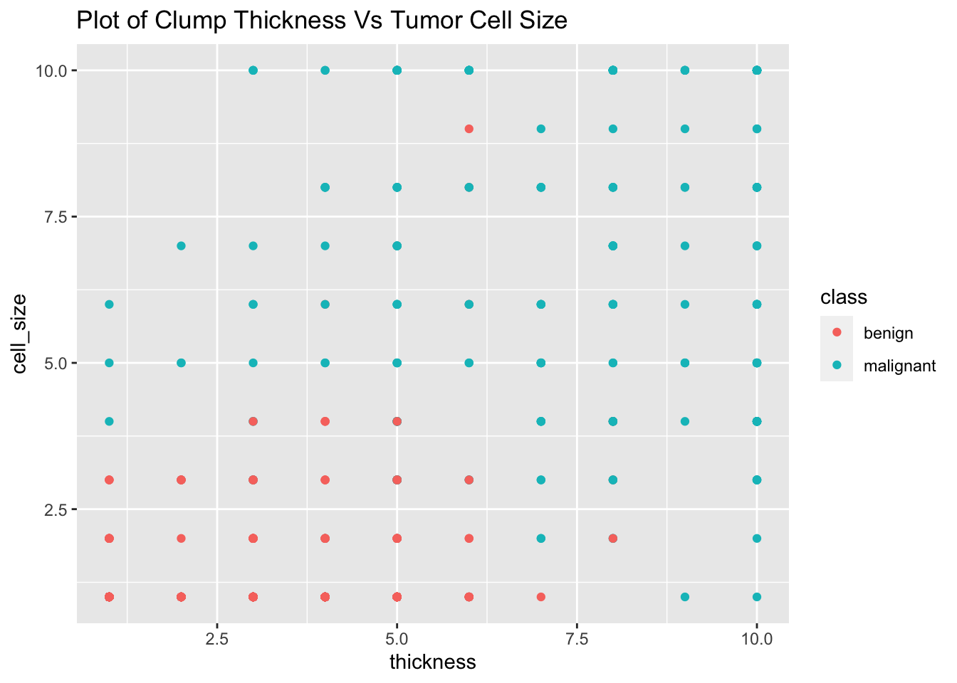
#normalize the bare nuclei values
biopsy_new<-filter(biopsy_new,thickness>5.5)

head(biopsy_new,5)
## # A tibble: 5 × 9
## ID thickness cell_size cell_shape marg_adhesion epithelial_cell_size
## <chr> <int> <int> <int> <int> <int>
## 1 1016277 6 8 8 1 3
## 2 1017122 8 10 10 8 7
## 3 1044572 8 7 5 10 7
## 4 1047630 7 4 6 4 6
## 5 1050670 10 7 7 6 4
## # … with 3 more variables: bare_nuclei <dbl>, norm_nucleoli <int>, class <fct>22.13 Arrange
Arrange reorders the rows of the data based on their contents in the ascending order by default.
The doctors would want to view the data in the order of the cell size of the tumor.
#arrange in the order of V2:cell size
arrange(biopsy_new,cell_size)
## # A tibble: 186 × 9
## ID thickness cell_size cell_shape marg_adhesion epithelial_cell_size
## <chr> <int> <int> <int> <int> <int>
## 1 1050718 6 1 1 1 2
## 2 1204898 6 1 1 1 2
## 3 1223967 6 1 3 1 2
## 4 543558 6 1 3 1 4
## 5 63375 9 1 2 6 4
## 6 752904 10 1 1 1 2
## 7 1276091 6 1 1 3 2
## 8 1238777 6 1 1 3 2
## 9 1257608 6 1 1 1 1
## 10 1224565 6 1 1 1 2
## # … with 176 more rows, and 3 more variables: bare_nuclei <dbl>,
## # norm_nucleoli <int>, class <fct>This shows the data in increasing order of the cell size.
To arrange the rows in decreasing order of V2, we add the desc() function to the variable before passing it to arrange.
#arrange in the order of V2:cell size in decreasing order
arrange(biopsy_new,desc(cell_size))
## # A tibble: 186 × 9
## ID thickness cell_size cell_shape marg_adhesion epithelial_cell_size
## <chr> <int> <int> <int> <int> <int>
## 1 1017122 8 10 10 8 7
## 2 1080185 10 10 10 8 6
## 3 1100524 6 10 10 2 8
## 4 1103608 10 10 10 4 8
## 5 1112209 8 10 10 1 3
## 6 1116116 9 10 10 1 10
## 7 1123061 6 10 2 8 10
## 8 1168736 10 10 10 10 10
## 9 1170419 10 10 10 8 2
## 10 1173216 10 10 10 3 10
## # … with 176 more rows, and 3 more variables: bare_nuclei <dbl>,
## # norm_nucleoli <int>, class <fct>As you can see, there are a number of rows with the same value of V2:cell_size. To break the tie, you can add another variable to be used for ordering when the first variable has the same value.
Here, we use the tie breaker as the order of variable V3: by cell shape and by ID:
#arrange in the order of V2:cell size
biopsy_new<-arrange(biopsy_new,desc(cell_size),desc(cell_shape),ID)

head(biopsy_new,5)
## # A tibble: 5 × 9
## ID thickness cell_size cell_shape marg_adhesion epithelial_cell_size
## <chr> <int> <int> <int> <int> <int>
## 1 1017122 8 10 10 8 7
## 2 1073960 10 10 10 10 6
## 3 1080185 10 10 10 8 6
## 4 1100524 6 10 10 2 8
## 5 1100524 6 10 10 2 8
## # … with 3 more variables: bare_nuclei <dbl>, norm_nucleoli <int>, class <fct>22.14 Summarize & Group By
Summarize uses the data to create a new data frame with the summary statistics such as minimum, maximum, average, and so on. These statistical functions must be aggregate functions which take a vector of values as input and output a single value.
The group_by function groups the data by the values of the variables. This, along with summarize, makes observations about groups of rows of the dataset.
The doctors would want to see the maximum cell size and the thickness for each of the classes: benign and malignant. This can be done by grouping the data by class and finding the maximum of the required variables:
biopsy_grouped <- group_by(biopsy_new,class)
summarize(biopsy_grouped, max(thickness), mean(cell_size), var(norm_nucleoli))
## # A tibble: 2 × 4
## class `max(thickness)` `mean(cell_size)` `var(norm_nucleoli)`
## <fct> <int> <dbl> <dbl>
## 1 benign 8 2.67 5.93
## 2 malignant 10 6.73 11.322.15 Pipe Operator
What if we want to use the various data wrangling verbs together?
This could be done by saving the result of each wrangling function in a new variable and using it for the next function as we did above. However, this is not recommended as:
It requires extra typing and longer code.
Unnecessary space is used up to save the various variables. If the data is large, this method slows down the analysis.
The pipe operator can be used instead for the same purpose. The operator is placed between and object and the function. The pipe takes the object on its left and passes it as the first argument to the function to its right.
The pipe operator is a part of the magrittr package. However, this package need not be loaded as the dplyr package makes life simpler and imports the pipe operator for us:
biopsy_grouped <- biopsy_new %>%
  group_by(class) %>%
  summarize(max(thickness),mean(cell_size),var(norm_nucleoli))

head(biopsy_grouped)
## # A tibble: 2 × 4
## class `max(thickness)` `mean(cell_size)` `var(norm_nucleoli)`
## <fct> <int> <dbl> <dbl>
## 1 benign 8 2.67 5.93
## 2 malignant 10 6.73 11.322.16 Tidying the transformed data
Have a look again at the messy data:
# Messy Data
head(biopsy_new,5)
## # A tibble: 5 × 9
## ID thickness cell_size cell_shape marg_adhesion epithelial_cell_size
## <chr> <int> <int> <int> <int> <int>
## 1 1017122 8 10 10 8 7
## 2 1073960 10 10 10 10 6
## 3 1080185 10 10 10 8 6
## 4 1100524 6 10 10 2 8
## 5 1100524 6 10 10 2 8
## # … with 3 more variables: bare_nuclei <dbl>, norm_nucleoli <int>, class <fct>Planning is required to decide which columns we need to keep unchanged, which ones to change, and what names are to be given to the new columns. The columns to keep are the ones that are already tidy. The ones to change are the ones that aren’t true variables but in fact levels of another variable.
So, the ID and class columns are already tidy. These are kept as is.
The columns V1:thickness, V2:cell_size, V3:cell_shape, V4:marg_adhesion, V5:epithelial_cell_size, V6:bare_nuclei, and V8:norm_nucleoli are not true variables but values of the variable Tumor_attributes.
We can fix this with tidyr::gather(), which is used to convert data from messy to tidy. The gather function takes the data frame which we want to tidy as input. The next two parameters are the names of the key and the value columns in the tidy dataset.
In our example, key=‘Tumor_Atrributes’ and value=‘Score’. You can also specify the columns that you do not want to be tidied, i.e. ID and class:
#Tidy Data
library(tidyr)
tidy_df <- biopsy_new %>% gather(key = "Tumor_Attributes", value = "Score", -ID, -class)

tidy_df
## # A tibble: 1,302 × 4
## ID class Tumor_Attributes Score
## <chr> <fct> <chr> <dbl>
## 1 1017122 malignant thickness 8
## 2 1073960 malignant thickness 10
## 3 1080185 malignant thickness 10
## 4 1100524 malignant thickness 6
## 5 1100524 malignant thickness 6
## 6 1103608 malignant thickness 10
## 7 1112209 malignant thickness 8
## 8 1116116 malignant thickness 9
## 9 1116116 malignant thickness 9
## 10 1168736 malignant thickness 10
## # … with 1,292 more rows22.17 Helpful Links
- r4ds on tidy data: It is always best to learn from the source, so a textbook written by Hadley Wickham is perfect.
- DataCamp dplyr course: This course covers the different fucntions in dplyr and how they manipulate data.
with