34 Animation graphs in plot_ly and gganimate
Yingtong Peng and Xiaoran Hu
Motivation: In classes, we have seen many data graphs that change over time, finding changes over time costs lots of graphing work since we need to draw one plot for each time, however, using animation plot, changes over time/groups can be seen in one plot easily and clearly. One of the advantages of animation is that it expands the number of variables we can visualize, and we can let the variables in the data set “drive” the animation.In this project, we learned two ways to draw animation plots: 1.Using plot_ly() function with ‘frame’ argument. 2.Using animate() function from ggplot. We also learned how to use animation options to make our graphic transitions smoother. Next time, we can further improve the animation plots: Change slider appearance, glyph color,shape,size, axis labels. We can also do other animation plots, such as dynamic box plot, dynamic map.
34.1 Types of graphics
- Static(Permanently fixed after it is created)
- Interactive(Changes based on the action performed by user)
- Dynamic(Changes periodically without user input)
34.2 Self-created data
theme_set(theme_pubr())
# Make 2 basic states and concatenate them:
dat1 <- data.frame(group=c("A","B","C"), values=c(3,5,9), frame=rep('a',3))
dat2 <- data.frame(group=c("A","B","C"), values=c(6,4,8), frame=rep('b',3))
data <- rbind(dat1,dat2)
head(data)
## group values frame
## 1 A 3 a
## 2 B 5 a
## 3 C 9 a
## 4 A 6 b
## 5 B 4 b
## 6 C 8 b34.2.1 Static Barplots(One categorical variable, One discrete variable over group)
# Static barplots:
g1<-ggplot(dat1, aes(x=group, y=values, fill=group)) +
  geom_bar(stat='identity')
g2<-ggplot(dat2, aes(x=group, y=values, fill=group)) +
  geom_bar(stat='identity')
figure<-ggarrange(g1,g2,labels=c("dat1","dat2"),legend="bottom",common.legend=TRUE)
figure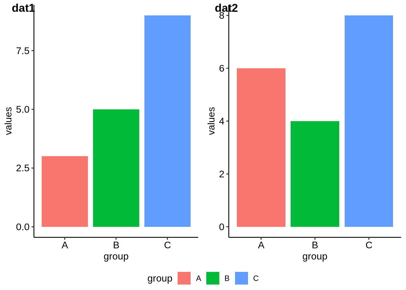
34.2.2 Dynamic Barplot(One categorical variable, One discrete variable over group)
# Make a dynamic ggplot,add frame=group
g3<-ggplot(data, aes(x=group, y=values, fill=group)) +
  geom_bar(stat='identity') +
  theme_bw() +
  # gganimate specific bits:
  transition_states(
    frame,
    transition_length = 2,
    state_length = 1
  ) +
  ease_aes('sine-in-out')
animate(g3,renderer=gifski_renderer())
Using dynamic plot, changes between two data sets can be seen and understood easily in one single plot.
34.3 GDP data
# Get data:
head(gapminder)
## # A tibble: 6 × 6
## country continent year lifeExp pop gdpPercap
## <fct> <fct> <int> <dbl> <int> <dbl>
## 1 Afghanistan Asia 1952 28.8 8425333 779.
## 2 Afghanistan Asia 1957 30.3 9240934 821.
## 3 Afghanistan Asia 1962 32.0 10267083 853.
## 4 Afghanistan Asia 1967 34.0 11537966 836.
## 5 Afghanistan Asia 1972 36.1 13079460 740.
## 6 Afghanistan Asia 1977 38.4 14880372 786.34.3.1 Animation Plot using gganimate(Two Continuous Variables Over Time)
# Make a dynamic ggplot, add frame=year: one image per year
g3<-ggplot(gapminder, aes(gdpPercap, lifeExp, size = pop, color = continent)) +
  geom_point() +
  scale_x_log10() +
  theme_bw() +
  # gganimate specific bits:
  labs(title = 'Year: {frame_time}', x = 'GDP per capita', y = 'life expectancy') +
  transition_time(year) +
  ease_aes('linear')
animate(g3,renderer=gifski_renderer())
### Animation Plot using plotly(Two Continuous Variables Over Time)
fig<-gapminder %>%
  plot_ly(x = ~gdpPercap, y = ~lifeExp, size = ~pop, color = ~continent, frame = ~year, text=~country, hoverinfo = "text", type = 'scatter', mode = 'markers' )  %>%
  add_text(x = 6500, y = 50, text = ~year, frame = ~year, textfont = list(size=150,color=toRGB("gray80")))
fig<-fig %>%
  layout( xaxis = list( type = "log" ) )
fig
34.3.2 Add Animation Options
fig<-fig %>%
  animation_opts(1000, easing = "elastic", redraw = FALSE)
fig
There are more easing options for animation:“linear”,“quad”,“cubic”,“sin”,“exp”,“circle”,“back”,“bounce”
34.3.3 Animation Plot facet by continent(Two Continuous Variables Over Time)
# Make a ggplot, but add frame=year: one image per year
g4<-ggplot(gapminder, aes(gdpPercap, lifeExp, size = pop, colour = country)) +
  geom_point(alpha = 0.7, show.legend = FALSE) +
  scale_colour_manual(values = country_colors) +
  scale_size(range = c(2, 12)) +
  scale_x_log10() +
  facet_wrap(~continent) +
  # Here comes the gganimate specific bits
  labs(title = 'Year: {frame_time}', x = 'GDP per capita', y = 'life expectancy') +
  transition_time(year) +
  ease_aes('linear')
animate(g4,renderer=gifski_renderer())
34.4 Babynames Data
head(babynames)## # A tibble: 6 × 5
## year sex name n prop
## <dbl> <chr> <chr> <int> <dbl>
## 1 1880 F Mary 7065 0.0724
## 2 1880 F Anna 2604 0.0267
## 3 1880 F Emma 2003 0.0205
## 4 1880 F Elizabeth 1939 0.0199
## 5 1880 F Minnie 1746 0.0179
## 6 1880 F Margaret 1578 0.016234.4.4 Animation Plot using gganimate(One categorical variable, one continuous variable over time)
# Plot
g5<-don %>%
  ggplot( aes(x=year, y=n, group=name, color=name)) +
    geom_line() +
    geom_point() +
    ggtitle("Popularity of American names in the previous 30 years") +
    theme_ipsum() +
    ylab("Number of babies born") +
    transition_reveal(year)
animate(g5,renderer=gifski_renderer())