31 wordcloud
Tianyi Lu (tl3089) and Xinyu Zhang (xz3054)
31.1 Motivation
After half-semester of learning in GR5293 Statistical Graphics, we have learned a lot in statistical Graphics with respect to numbers. However, we think we also need some graphs to show the statistical visualization for text. So we want to find a supreme visually appealing way to show the main information in the text. We decided to focus on wordcloud.
We have many ways to visualize numbers, what about words, what can we use to visualize words. After our research, we found two packages, wordcloud and ggwordcloud, to show the frequency of words. It is a text visualization tool to statistically show the frequency of the word.
After we learned this topic. we also find some pros and cons of wordclouds.
For pros of Word clouds, you can easily extract the insights to draw the discussions over the problem. Through the highlighted text, it facilitates the text analysis to understand the behaviour and sentiment of the data.
For cons of Word clouds, you cannot use the word clouds for the quantitative or numerical data analysis as this process only includes the categorical data. And the wordclouds will fail in the process of major decision making.
In the future application, we think we can apply it to analyze the same event reported by different countries, such as the COVID-19 news in different countries. By using this tool, we can see the different attitudes toward the same event from different parties.
In this Community contribution, we will introduce two ways to draw Wordcloud graphs. The first way is using wordcloud2 package. The second way is using ggwordclod package under ggplot2. This is used to show the frequency of the presence of words in the text.
Tianyi Lu works for the first part, which is the worldCloud2 Method.
Xinyu Zhang works for the second part, which is the ggwordcloud Method.
And we collaborated to give the third part of a complete example to show how to fulfil the word visual representation.
31.2 worldCloud2 Method
wordcloud2: this package provides an HTML5 interface to wordcloud for data visualization.
This document show two main function in Wordcloud2:
- wordcloud2: provide traditional wordcloud with HTML5
- letterCloud: provide wordcloud with selected word(letters).
31.2.1 Arguments
data - A data frame including word and freq in each column
size - Font size, default is 1. The larger size means the bigger word.
fontFamily - Font to use.
fontWeight - Font weight to use, e.g. normal, bold or 600
color - color of the text, keyword ‘random-dark’ and ‘random-light’ can be used. color vector is also supported in this param
minSize - A character string of the subtitle
backgroundColor - Color of the background.
gridSize - Size of the grid in pixels for marking the availability of the canvas the larger the grid size, the bigger the gap between words.
minRotation - If the word should rotate, the minimum rotation (in rad) the text should rotate.
maxRotation - If the word should rotate, the maximum rotation (in rad) the text should rotate. Set the two value equal to keep all text in one angle.
rotateRatio - Probability for the word to rotate. Set the number to 1 to always rotate.
shape - The shape of the “cloud” to draw. Can be a keyword present. Available presents are ‘circle’ (default), ‘cardioid’ (apple or heart shape curve, the most known polar equation), ‘diamond’ (alias of square), ‘triangle-forward’, ‘triangle’, ‘pentagon’, and ‘star’.
ellipticity - degree of “flatness” of the shape wordcloud2.js should draw.
figPath - The path to a figure used as a mask
widgetsize - size of the widgets
31.3 worldCloud2 Example:
data=demoFreq
wordcloud2(data=demoFreq)
31.3.1 Operations that used most frequently
31.3.1.1 Change the size of these words
wordcloud2(data = demoFreq, size = 0.5)31.3.1.2 Change the text colors and background colors:
wordcloud2(data = demoFreq,color="random-light",backgroundColor = "orange")31.3.1.3 Customize colors
wordcloud2(demoFreq,
  color = ifelse(demoFreq[, 2] > 20, 'orange', 'skyblue'))
colorVec = rep(c('red', 'skyblue'), length.out=nrow(demoFreq))
wordcloud2(demoFreq, color = colorVec, fontWeight = "bold")
Difference between above teo methods: The first way to change the color is according to our requirement, when the frequency of word is greater than 20, the word is orange and the rest is skyblue.
The second way is to assign red and blue to each word one by one. If you want to show the frequency of words more clearly, we recommend using the first method.
31.3.1.4 Change the rotation of the words:
wordcloud2(data = demoFreq,minRotation = -pi/2, maxRotation = -pi/2)31.3.1.5 Change word cloud shape
There are several word cloud shape under the wordcloud2 package, such as circle, diamond, cardioid, triangle. We can use it by add a shape command.
##There are several word cloud shape under the wordcloud2 package
wordcloud2(demoFreq, size = 0.3, shape = 'circle')
wordcloud2(demoFreq, size = 0.3, shape = 'triangle-forward')
wordcloud2(demoFreq, size = 0.3, shape = 'pentagon')
wordcloud2(demoFreq, size = 0.3, shape = 'star')31.3.1.6 Use an user-defined letter or text as shape
letterCloud(demoFreq, word = "GR5293", wordSize = 1)31.3.1.7 Use figure file as a mask
fig = system.file("examples/t.png", package = "wordcloud2")
wordcloud2(demoFreq, figPath = fig, size = 1.5)
31.4 ggwordcloud Method
ggwordcloud provides a word cloud text geom for ggplot2. The cloud can grow according to a shape and stay within a mask. The size aesthetic is used either to control the font size or the printed area of the words. ggwordcloud also supports arbitrary text rotation. The faceting scheme of ggplot2 can also be used. Two functions meant to be the equivalent of wordcloud and wordcloud2 are proposed.
geom_text_wordcloud: it adds text to the plot using a variation of the wordcloud2.js algorithm. The texts are layered around a spiral centered on the original position
geom_text_wordcloud_area: it is an alias, with a different set of default, that chooses a font size so that the area of the text is now related to the size aesthetic.
31.4.1 Arguments
words - the words
freq - their frequencies
scale - A vector of length 2 indicating the range of the size of the words.
min.freq - words with frequency below min.freq will not be plotted
max.words - Maximum number of words to be plotted. least frequent terms dropped
random.order - plot words in random order. If false, they will be plotted in decreasing frequency
random.color - choose colors randomly from the colors. If false, the color is chosen based on the frequency
rot.per - proportion words with 90 degree rotation
colors - color words from least to most frequent
ordered.colors - if true, then colors are assigned to words in order
31.5 ggwordclod Example:
#install.packages("ggwordcloud")
#install.packages("showtext")

data <- mtcars
data$name <- row.names(mtcars)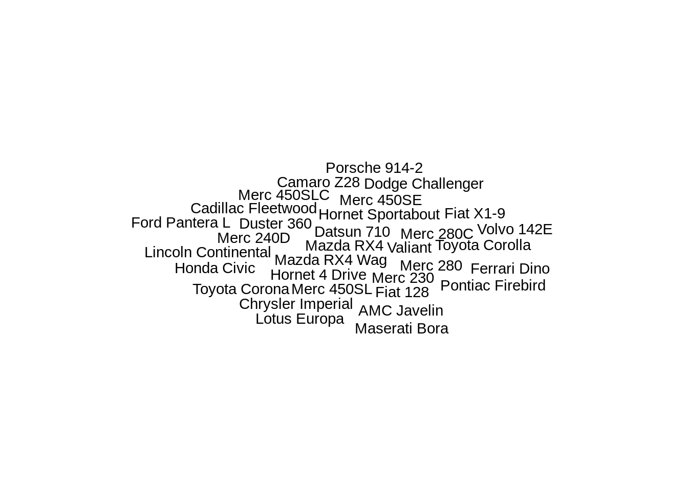
31.5.2 Text Size
The geom_text_wordcloud geom constructs a word cloud from a list of words given by the label aesthetic. The default is the words had the same size because we do not specify a size aesthetic. If we want high frequency words have larger size, we should chang “size” value.
data$size <- data$mpg
data$size[c(1,4)] <- data$size[c(1,4)] + 100

ggplot(data, aes(label = name, size = size)) +
  geom_text_wordcloud() +
  theme_minimal()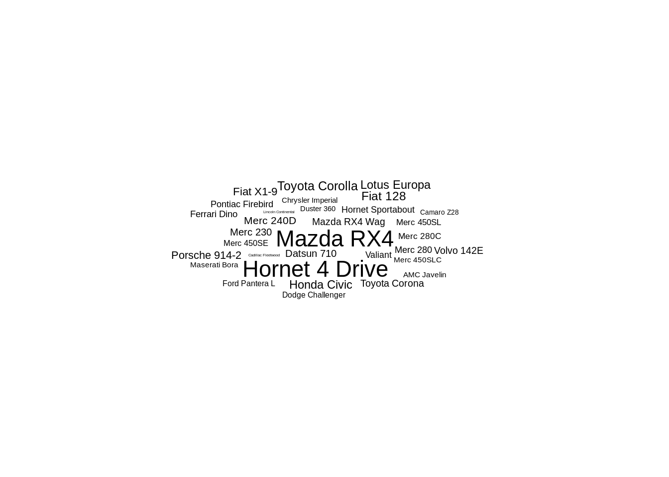
31.5.3 text area
Text area by default is a natural choice for a shape as the area of the shape will be proportional to the raw size aesthetic but not necessarily for texts with different lengths. In ggwordcloud2, there is an option, area_corr to scale the font of each label so that the text area is a function of the raw size aesthetic when used in combination with scale_size_area:
ggplot(data, aes(label = name, size = size)) +
  geom_text_wordcloud(area_corr = T) +
  scale_size_area(max_size = 10) +
  theme_minimal()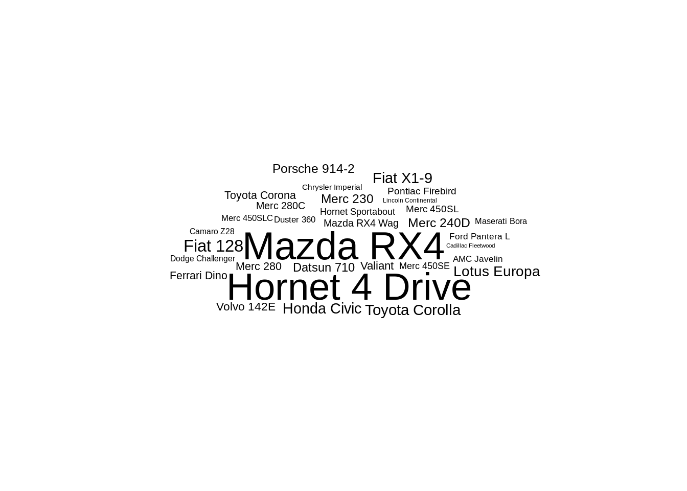
One can equivalently use the geom_text_wordcloud_area geom:
ggplot(data, aes(label = name, size = size)) +
  geom_text_wordcloud_area() +
  scale_size_area(max_size = 10) +
  theme_minimal()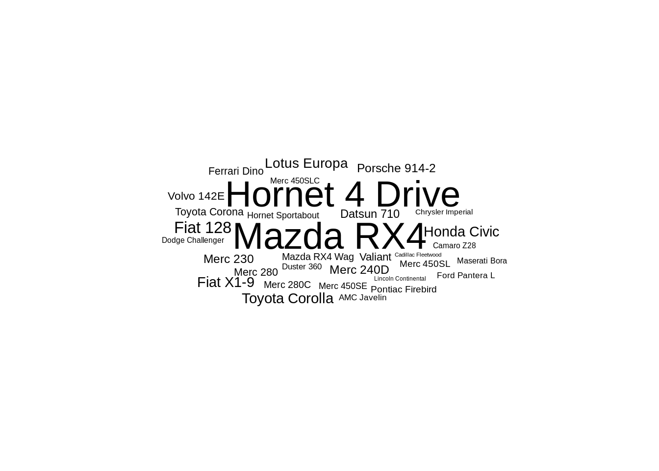
31.5.4 rotation
data$rot <- 90*(runif(nrow(data))>.6)
ggplot(data = data, aes(label = name, size = size, angle = rot)) +
  geom_text_wordcloud() +
  scale_size(range = c(2,12)) +
theme_minimal() 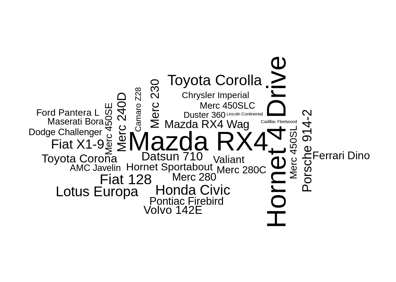
31.5.5 eccentricity
The ggwordcloud algorithm moves the text around a spiral until it finds a free place for it. This spiral has by default a vertical eccentricity of .65, so that the spiral is 1/.65 wider than taller.
ggplot(data = data, aes(label = name, size = size, angle = rot)) +
  geom_text_wordcloud()  +
  scale_size(range = c(2,12)) +
theme_minimal() 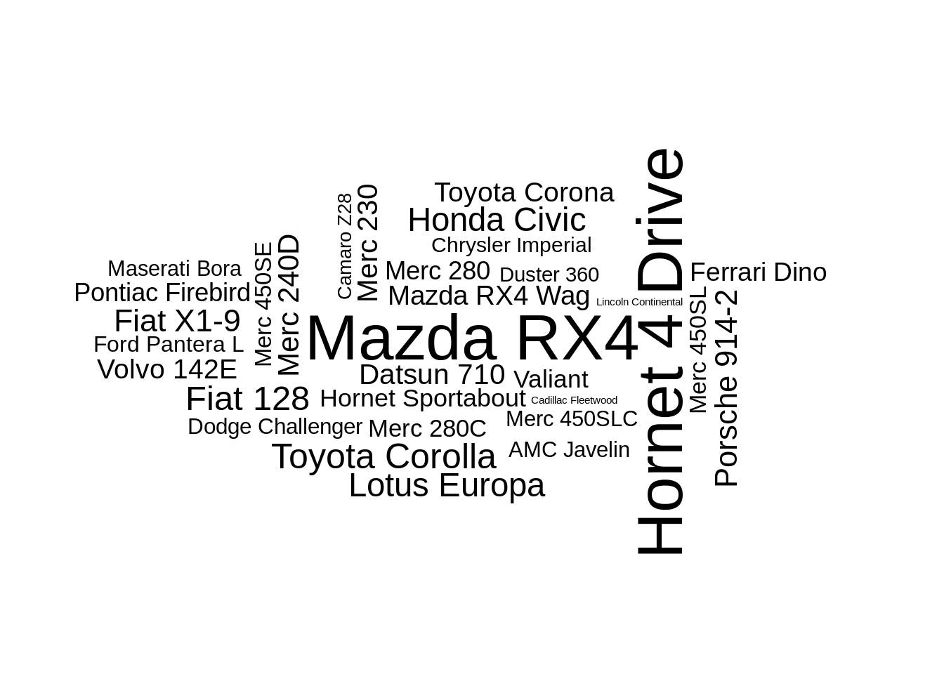
This can be changed using the eccentricity parameter:
ggplot(data = data, aes(label = name, size = size, angle = rot)) +
  geom_text_wordcloud(eccentricity = 1)  +
  scale_size(range = c(2,12)) +
theme_minimal() 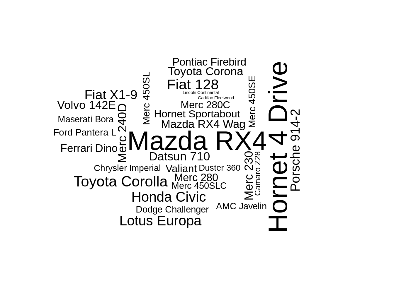
31.5.6 Shape
The base shape of ggwordcloud is a circle: the words are place by following a circle spiral. This base shape circle can be change to others (cardioid, diamond, square, triangle-forward, triangle-upright, pentagon or star) using the shape option.
set.seed(42)
ggplot(data, aes(label = name, size = size)) +
    geom_text_wordcloud_area(shape = "star") +
    scale_size_area(max_size = 5) +
    theme_minimal()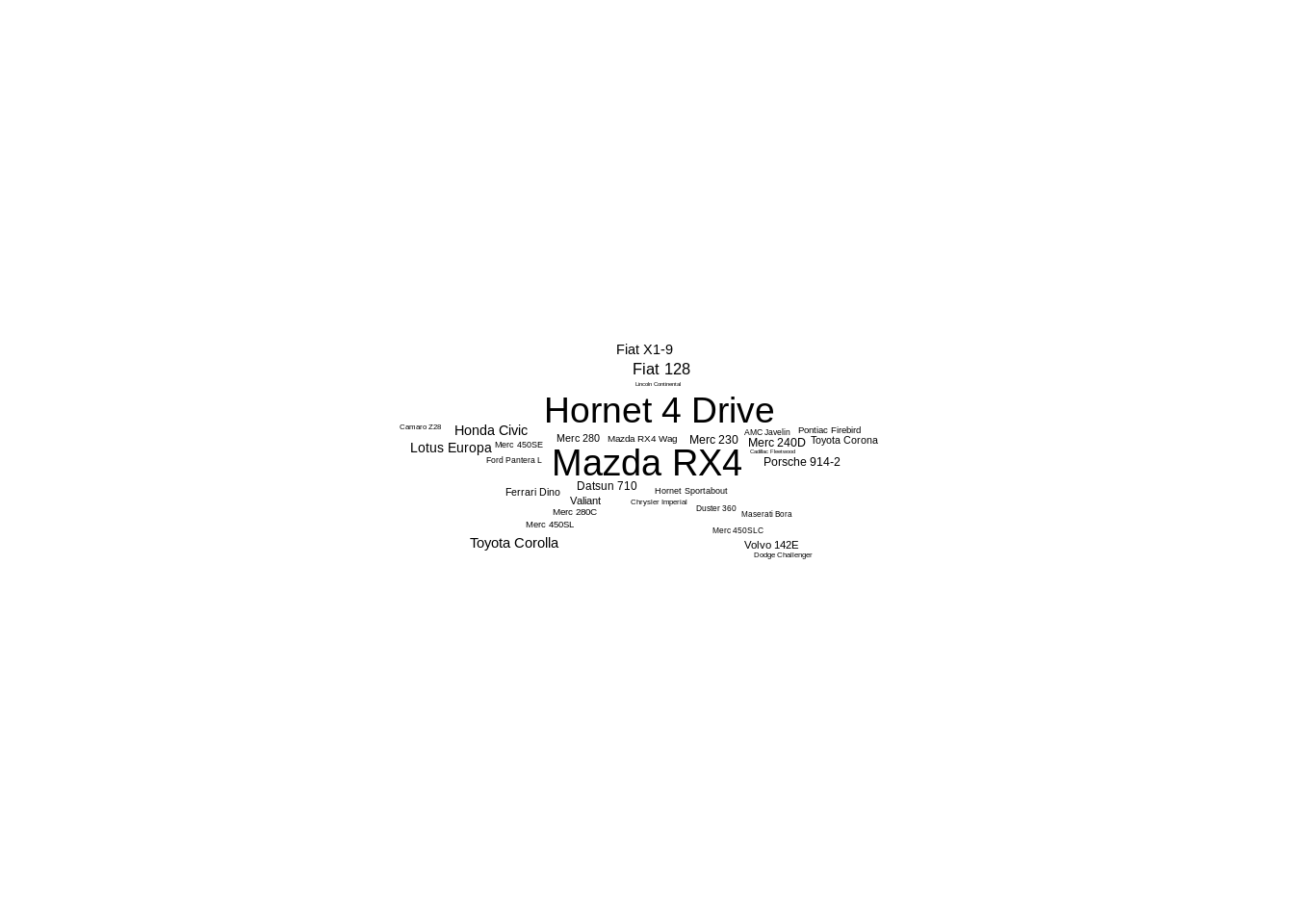
31.5.7 Color
ggplot(data,aes(label = name, size = size, color = factor(sample.int(10, nrow(data), replace = TRUE)),angle = rot)) +
  geom_text_wordcloud_area() +
  scale_size_area(max_size = 5) +
  theme_minimal()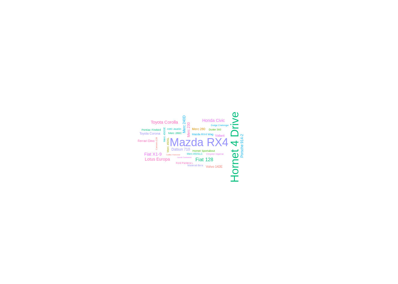
31.6 A complete example to show how to fulfil the word visual representation
Before doing the word visualization, it is important to cover a few terms:
Corpus - A list of blocks of text (the column speechtext in the object sotu is our corpus).
Document - These are the separate blocks of text from the corpus.
Term- These are the individual words that make up each document, sometimes called unigrams. The document is broken apart at the spaces (each word in a cell in column speechtext in object sotu is a term).
articles<-read.csv("resources/wordcloud/articles.csv")#The data set is downloaded from Kaggle, and the link is provided in the reference list.31.6.1 Create a corpus from actual text
articles.corpus=Corpus(VectorSource(articles$title))
removeHTML=function(text){
  text=gsub(pattern='<.+\\">','',text)
  text=gsub(pattern='</.+>','',text)
  return(text)
}31.6.3 Creat term document matrix
tdm=TermDocumentMatrix(articles.corpus)%>%#each row represent a word, and each column represent the document and the cell correspond how many times the word appears in the document
as.matrix()#convert it into a R matrix we can work with
words=sort(rowSums(tdm),decreasing = TRUE)
df=data.frame(word=names(words),freq=words)
31.6.4 Minor adjustments to data frame
df=df%>%
  filter(nchar(as.character(word))>2,
         word!="don'")
31.6.5 Create word cloud
wordcloud2(df)