40 Calendar heat map tutorial
Eva Dai
Hi there! Here I want to share with you a way of creating calendar heat map for multiple years. Calendar heat map is a calendar that uses colored cells to show the relative number of a variable. The final project of our group is focused on the waiting time of the rides in Disney World. Since the data is highly related to time, I find that calendar heat map can be a good way of representing data from multiple years. In this calendar heat map tutorial, I will show how to plot two types of calendar heat maps, one for data from multiple years and one for a single year.
library(lubridate)
library(tidyverse)
library(dplyr)
library(zoo)
library(gridExtra)
library(ggplot2)
library(calendR)
I. Data processing: date transformation The original data set comes from the touringplans.com, under the ride “Soarin’”. The data is very large and has 274770 rows. The values for waiting time are scattered in two columns. So first of all we clean them and merge the two columns. And then we choose “datetime” which represents the date and time, and “SPOSTMIN” that represents the waiting time documented. And in order to learn more from this tutorial, I will start with transforming time values accurate to seconds, so the “datetime” column is selected.
soarin <- readr::read_csv("https://cdn.touringplans.com/datasets/soarin.csv", show_col_types = FALSE)
head(soarin)
## # A tibble: 6 × 4
## date datetime SACTMIN SPOSTMIN
## <chr> <dttm> <dbl> <dbl>
## 1 01/01/2015 2015-01-01 07:45:15 NA 10
## 2 01/01/2015 2015-01-01 07:52:16 NA 10
## 3 01/01/2015 2015-01-01 08:03:17 NA 10
## 4 01/01/2015 2015-01-01 08:10:16 NA 35
## 5 01/01/2015 2015-01-01 08:17:19 NA 45
## 6 01/01/2015 2015-01-01 08:24:16 NA 35
for (i in 1:nrow(soarin)){
  if(is.na(soarin$SPOSTMIN[i]==T)){soarin$SPOSTMIN[i] <- soarin$SACTMIN[i]}
}
df <- soarin %>% select(-c(SACTMIN,date)) %>% filter(SPOSTMIN>0)
head(df)
## # A tibble: 6 × 2
## datetime SPOSTMIN
## <dttm> <dbl>
## 1 2015-01-01 07:45:15 10
## 2 2015-01-01 07:52:16 10
## 3 2015-01-01 08:03:17 10
## 4 2015-01-01 08:10:16 35
## 5 2015-01-01 08:17:19 45
## 6 2015-01-01 08:24:16 35If the date information we get in the data file is more accurate than just date, we need to first transform it
We can use the zoo package to easily transform into date format
## # A tibble: 6 × 3
##   datetime            SPOSTMIN date
##   <dttm>                 <dbl> <date>
## 1 2015-01-01 07:45:15       10 2015-01-01
## 2 2015-01-01 07:52:16       10 2015-01-01
## 3 2015-01-01 08:03:17       10 2015-01-01
## 4 2015-01-01 08:10:16       35 2015-01-01
## 5 2015-01-01 08:17:19       45 2015-01-01
## 6 2015-01-01 08:24:16       35 2015-01-01
Then we need to calculate the daily average of the waiting time in order to make a calendar heatmap.
To create a calendar heatmap, we need to first create variables such as weekday, year, month, week, and week of month. Here I use the “lubridate” package that helps to calculate the day os a week for each date in the data frame.
wday() calculates the weekday of a given date. with label=TRUE, the output will be in verbal format, such as “Sun”, “Mon”, etc. Otherwise, the number of the weekday from 1 to 7 will be calculated
Similarly, year() calculates the year of the date and month() calculates the month of the date.
strftime() converts the date into the week number. With format=“%V”, week of the year from 1-53 will be given with Monday as the start of the week. Since we use Sunday as the start of the week, we need to add 1 into the function
new$week <- strftime(new$date+1, format = "%V")Since it is hard to find an R package that calculates the week of month, I created a function that takes date as an input. The function takes Sunday as the start of the week and the output will be an integer value specifying the week number of the month that the given date is on.
weekofmonth <- function(date){
  out <- as.integer(strftime(date, format = "%U"))-as.integer(strftime(floor_date(date, unit="months"), format = "%U"))+1
  return(out)
}

new$weekofmonth <- factor(weekofmonth(new$date))
We are now done with data processing. The data frame now includes all the factors we need for plotting.
head(new)## # A tibble: 6 × 7
## date mean_everyday weekday year month week weekofmonth
## <date> <dbl> <ord> <fct> <ord> <chr> <fct>
## 1 2015-01-01 89.6 Thu 2015 Jan 01 1
## 2 2015-01-02 81.1 Fri 2015 Jan 01 1
## 3 2015-01-03 73.4 Sat 2015 Jan 01 1
## 4 2015-01-04 58.1 Sun 2015 Jan 02 2
## 5 2015-01-05 58.4 Mon 2015 Jan 02 2
## 6 2015-01-06 55.6 Tue 2015 Jan 02 2- Plotting Calendar heat map
First we create the calendar heat map for all years in the data frame. The blanks on the graph is because of the missing of data for specific dates in the data frame.
ggplot(new, aes(weekday, fct_rev(weekofmonth), fill = mean_everyday)) +
  geom_tile(colour = "white") +
  facet_grid(year~month) +
  scale_fill_gradient(low="#FFE6EE" , high="#bb1919") +
  ggtitle("Calendar Heatmap")+
  xlab("Weekday")+labs(fill="Average Waiting Time")+
  ylab("Week Number")+
  scale_x_discrete(label=function(x) {abbreviate(x, minlength=1, strict = T)})+
  theme(axis.text=element_text(size=4))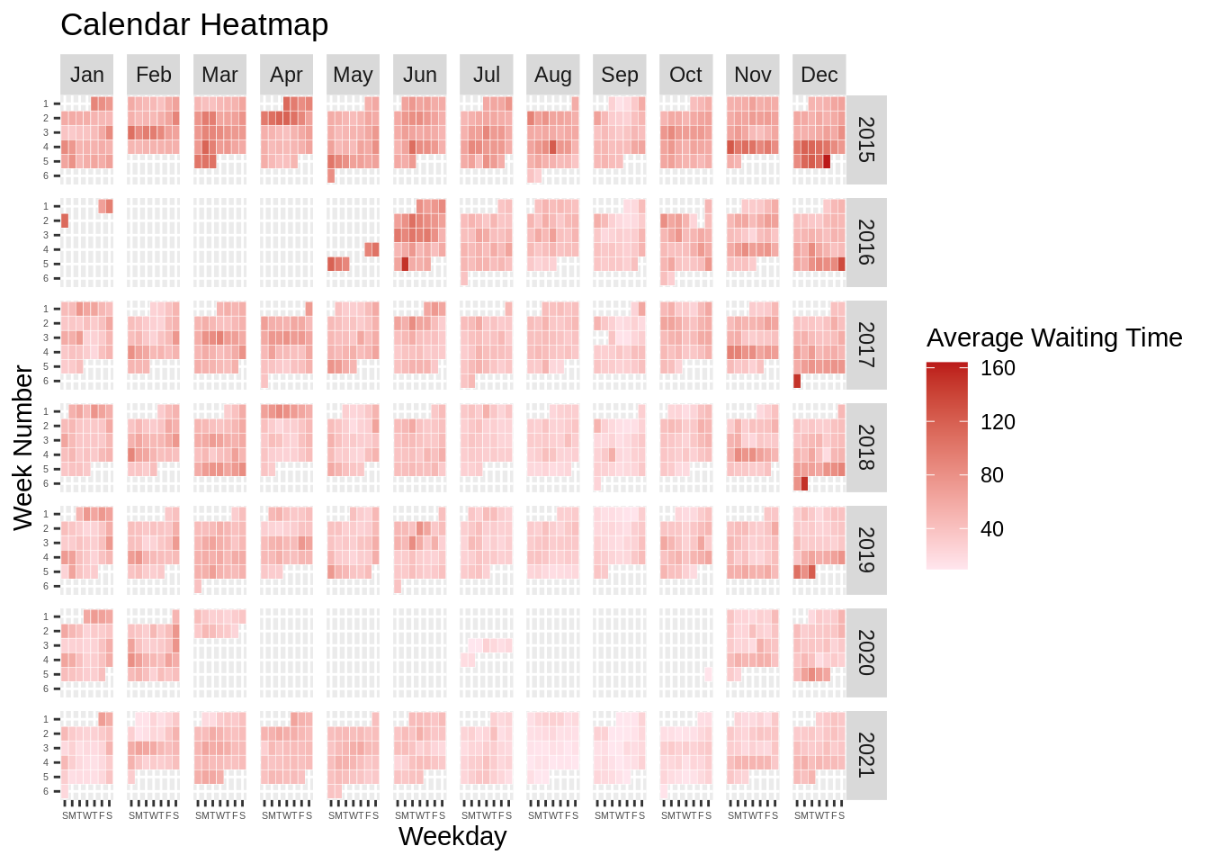
From the calendar heat map for the “Soarin’” ride of Disney World, we can easily see which days have a high average waiting time and which days have a low waiting time. And by comparing different levels of color fill over years, we can see the overall waiting pattern during a year and find which months have lower average waiting time. And we can also compare across years to see the overall crowdness of the year. For instance, the color fills for year 2021 are lighter than the other years, which can be considered directly impacted by the current pandemic.
If we want to take a closer look and create a heat map for a specific year from the dataframe, we can plot using the following code. Here we take 2015 as an example.
y <- 2015

ggplot(new%>%filter(year==y), aes(weekday, fct_rev(weekofmonth), fill = mean_everyday)) +
  geom_tile(colour = "white") +
  facet_wrap(~month) +
  scale_fill_gradient(low="#FFE6EE", high="#bb1919") +
  ggtitle("Calendar Heatmap")+
  xlab("Weekday")+labs(fill="Average Waiting Time")+
  theme(axis.text=element_text(size=6))+
  ylab("Week Number")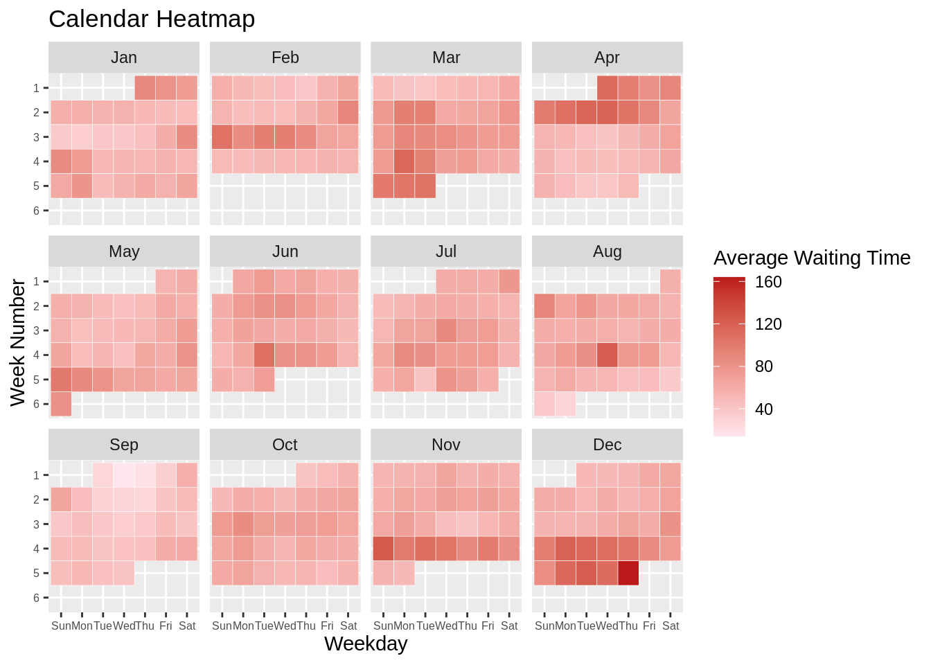
For a faster processing of the data into a calendar heatmap, we can use the package “calendR”. The package automatically creates the calendar of a specific year (or month), and fills color with values from the dataframe. We can specify the low and high colors and the colors to be filled in will be specified in “special.days”. For instance, we can create a similar calendar heatmap for year 2015.
calendR(year=2015, start="S",
        special.days = (new%>%filter(year==2015))$mean_everyday,
        gradient=TRUE,
        low.col="#f9d7d7",
        special.col="#bb1919",
        legend.pos = "right",
        legend.title = "Average Waiting Time",
        weeknames.size=2.5,
        day.size=2)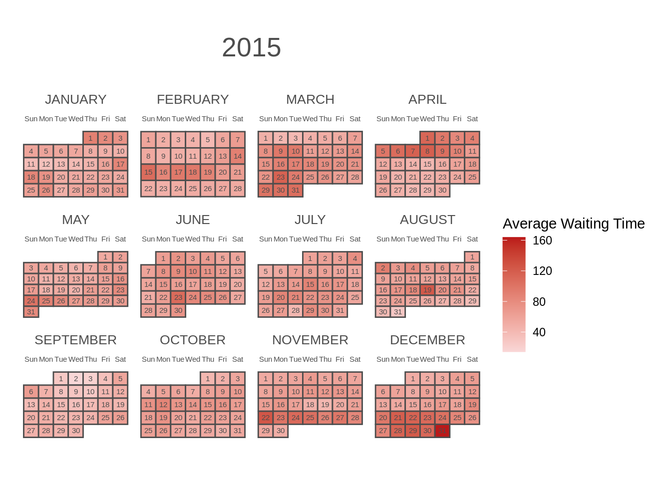
However, the package can create a calendar heatmap for at most a year. If we want to create a heatmap using all years from the data, we still need to plot using ggplot as drawn above.
As we can see, calendar heat map can be an efficient way of visualizing the variable value that we want to represent. And I hope this tutorial can be helpful!
References
https://touringplans.com/walt-disney-world/crowd-calendar#DataSets
https://stackoverflow.com/questions/25199851/r-how-to-get-the-week-number-of-the-month
https://stackoverflow.com/questions/48301514/r-fit-heat-map-into-grid-lines-on-calendar-heatmap
https://r-charts.com/evolution/monthly-calendar-heatmap/