32 Linear Modeling Using R via a Soccer Example
Fahad Alkhaja
32.1 Introduction
The goal of this assignment and tutorial is to show how one can use linear models in R to describe trends and be used as a predictive measure of future performance.
A commonly used model in the soccer world is that of xG, which roughly translates to the Expectation of a Goal being scored. \(E(Goal) =\)xG.
It is based on a probabilistic measure being assigned to each shot taken where each shot has an xG value based on likelihood of scoring from where the shot was taken. The xG values are thus tallied for a team. Thus, comparing xG values for teams over the course of a game or year can serve as a good indication of team performance without results bias and excluding for the most part luck, which in a low scoring game such as soccer plays a big factor.
Today, we will be exploring a more niche aspect of the expectations world in soccer. We will look to model the number of goals conceded based on some different parameters which include xGA expected goals against, or expected goals conceded, and some other defensive metrics such as Blocks, Tackles, and Pressures. This can help be a guide to see which factor is the most contributing to a team’s defensive record, in terms of goals conceded. Eventually this could be used to compare to that of the league table.
32.2 Data Loading
The Data used here is obtained directly from the FBref website under the Premier League 2021/22 season so far as of Mar 28, 2021 (1).
league_table <- read_xlsx("resources/linear_models_soccer_example/PL21-22_Points.xlsx",
                          skip = 0)
# Squad Standard Stats 2021-22 Premier League Table on FBRef

defense <- read_xlsx("resources/linear_models_soccer_example/PL21-22_Defense.xlsx",skip = 1)
# Squad Defensive Actions 2021-22 Premier League Table on FBRef
32.3 Data Wrangling
We have to then clean and prepare the relevant data so we can come up with appropriate models.
league_table_2 <- league_table %>%
  select(Rk:`xGD/90`) %>%
  mutate(`xGA/90` = round(xGA/MP, 3),
         PPG = round(Pts/MP, 3)) %>%
  select(-c(W,D,L))

defense_2 <- defense %>%
  select(-(`# Pl`)) %>%
  select(-(`TklW`:Past)) %>%
  select(-(Sh:Pass)) %>%
  rename(Tackles = `Tkl...4`,
         Pressures = Press,
         SuccPress = Succ,
         `%SuccPress` = `%`,
         Press_Def = `Def 3rd...16`,
         Press_Mid = `Mid 3rd...17`,
         Press_Att = `Att 3rd...18`) %>%
  select(-c(`Tkl+Int`))

defense_stats_cleaned <- league_table_2 %>%
  full_join(defense_2, by = "Squad") %>%
  select(-c(`90s`, GF, GD, xG, xGD, `xGD/90`))

defense_stats_cleaned
## # A tibble: 20 × 19
## Rk Squad MP GA Pts xGA `xGA/90` PPG Tackles Pressures
## <dbl> <chr> <dbl> <dbl> <dbl> <dbl> <dbl> <dbl> <dbl> <dbl>
## 1 1 Manchester Ci… 29 18 70 21.2 0.731 2.41 387 3265
## 2 2 Liverpool 29 20 69 27.6 0.952 2.38 422 4014
## 3 3 Chelsea 28 19 59 24.8 0.886 2.11 480 3989
## 4 4 Arsenal 28 31 54 34.2 1.22 1.93 430 3458
## 5 5 Tottenham 29 36 51 32.5 1.12 1.76 532 4348
## 6 6 Manchester Utd 29 40 50 41.3 1.42 1.72 481 3802
## 7 7 West Ham 30 39 48 38.6 1.29 1.6 466 3881
## 8 8 Wolves 30 26 46 42.9 1.43 1.53 579 4317
## 9 9 Aston Villa 29 40 36 36.6 1.26 1.24 524 4036
## 10 10 Leicester City 27 46 36 46.3 1.72 1.33 542 4234
## 11 11 Southampton 29 45 35 41.4 1.43 1.21 506 4366
## 12 12 Crystal Palace 29 38 34 34.2 1.18 1.17 567 4670
## 13 13 Brighton 29 36 33 37.3 1.29 1.14 566 4313
## 14 14 Newcastle Utd 29 49 31 42.5 1.47 1.07 532 4095
## 15 15 Brentford 30 47 30 39.3 1.31 1 560 4372
## 16 16 Leeds United 30 67 29 55 1.83 0.967 650 5224
## 17 17 Everton 27 47 25 39.3 1.46 0.926 576 4477
## 18 18 Watford 29 55 22 49.6 1.71 0.759 535 4422
## 19 19 Burnley 27 38 21 39.2 1.45 0.778 465 3899
## 20 20 Norwich City 29 63 17 55.5 1.91 0.586 528 4626
## # … with 9 more variables: SuccPress <dbl>, `%SuccPress` <dbl>,
## # Press_Def <dbl>, Press_Mid <dbl>, Press_Att <dbl>, Blocks <dbl>, Int <dbl>,
## # Clr <dbl>, Err <dbl>32.4 Initial Model Fit: Simple Linear Model (one variable)
Now that we have cleaned the data to only the relevant defensive metrics that we will be exploring, we can get to work.
First we will attempt to fit a linear model (lm) using only xGA to estimate xG.
The “lm” function takes the “formula” argument in the form y~x such that it runs a linear regression with the equation \[ y = \beta_0 + \beta_1x\]. In the case of more parameters the equation takes the same linear form : \[y = \beta_0 + \beta_1x_1 + \beta_2x_2 + ... + \beta_nx_n\].
As seen below, the lm(…) function serves to find the best estimates for each \(\beta\). Running the function summary(lm(…)) as such gives a much more detailed view including standard errors of such estimations.
# running lm on the model finds the best estimates for beta_0 (the intercept)
# and beta_1 in this case.

model_1 <- lm(formula = GA ~ xGA, data = defense_stats_cleaned)

model_1
##
## Call:
## lm(formula = GA ~ xGA, data = defense_stats_cleaned)
##
## Coefficients:
## (Intercept) xGA
## -13.00 1.36##
## Call:
## lm(formula = GA ~ xGA, data = defense_stats_cleaned)
##
## Residuals:
## Min 1Q Median 3Q Max
## -19.3528 -2.3693 0.5201 4.2639 6.5443
##
## Coefficients:
## Estimate Std. Error t value Pr(>|t|)
## (Intercept) -13.005 6.143 -2.117 0.0485 *
## xGA 1.360 0.154 8.836 5.79e-08 ***
## ---
## Signif. codes: 0 '***' 0.001 '**' 0.01 '*' 0.05 '.' 0.1 ' ' 1
##
## Residual standard error: 5.919 on 18 degrees of freedom
## Multiple R-squared: 0.8126, Adjusted R-squared: 0.8022
## F-statistic: 78.07 on 1 and 18 DF, p-value: 5.79e-08We can see that the intercept has a large variation. Inherently also, the value does not make sense because teams starting with an xGA of 0 will have an estimated GA of around -13.
We can also visualize this initial model with a simple scatter plot and a best fit line and an ideal model line, where GA = xGA, it is a perfect assumption.
defense_stats_cleaned %>%
  ggplot(aes(xGA, GA)) +
  geom_point() +
  geom_smooth(method='lm', formula= y~x, aes(color = "GA = -13.005 + 1.360 xGA")) +
  geom_abline(slope = 1, intercept = 0) +
  theme_bw() +
  labs(title = "Goals Conceded (GA) Estimated by xGA",
       subtitle = "There is a lot of variance around the estimated best fit line.",
       x = "xGA: Expected Goals Against",
       y = "GA : Goals Against",
       color = "") +
  theme(legend.position = "bottom")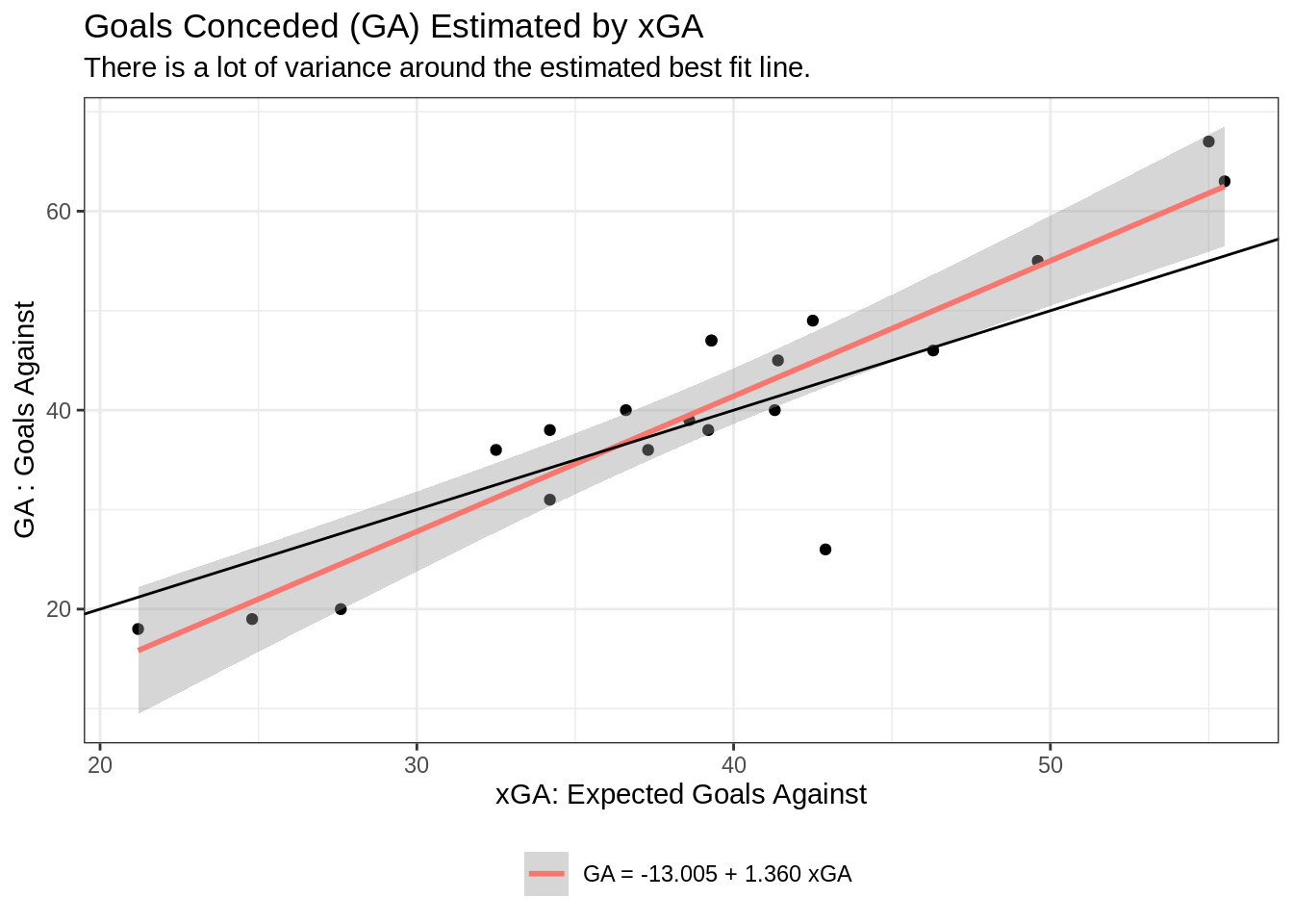
It is immediately clear that the simple model we ran is not sufficient, so how can we improve it?
32.5 Linear Model: Removing Intercept Term
First, we can get rid of the intercept because fundamentally in our problem here it does not make sense.
Adding a -1 at the end of the formula gets rid of the intercept term. such that formula = y ~ x - 1.
model_2 <- lm(formula = GA ~ xGA - 1, data = defense_stats_cleaned)

model_2
##
## Call:
## lm(formula = GA ~ xGA - 1, data = defense_stats_cleaned)
##
## Coefficients:
## xGA
## 1.042##
## Call:
## lm(formula = GA ~ xGA - 1, data = defense_stats_cleaned)
##
## Residuals:
## Min 1Q Median 3Q Max
## -18.7042 -3.3006 0.3178 3.6637 9.6870
##
## Coefficients:
## Estimate Std. Error t value Pr(>|t|)
## xGA 1.04206 0.03608 28.88 <2e-16 ***
## ---
## Signif. codes: 0 '***' 0.001 '**' 0.01 '*' 0.05 '.' 0.1 ' ' 1
##
## Residual standard error: 6.439 on 19 degrees of freedom
## Multiple R-squared: 0.9777, Adjusted R-squared: 0.9766
## F-statistic: 834.1 on 1 and 19 DF, p-value: < 2.2e-16
defense_stats_cleaned %>%
ggplot(aes(xGA, GA)) +
geom_point() +
geom_smooth(method='lm', formula= y~x-1, aes(color = "GA = 1.042xGA")) +
geom_abline(slope = 1, intercept = 0) +
theme_bw() +
labs(title = "Goals Conceded (GA) Estimated by xGA",
subtitle = "The best-fit line (Red) and Perfect Model Line are now much closer.",
x = "xGA: Expected Goals Against",
y = "GA : Goals Against",
color = "") +
theme(legend.position = "bottom")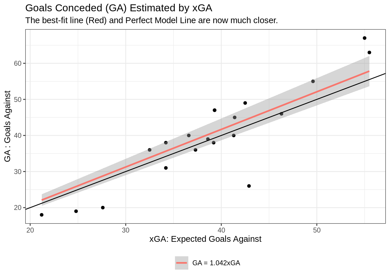 The line does seem to fit the ideal model line very well. However, there are still alot of data points quite spread it. So it is definitely worth exploring more parameters to see which one best fits our current data.
32.6 Additional Linear Parameters and Interactions
There are several methods to do this. We can add more linear terms and have our pick from any of the defensive metrics we narrowed down earlier. In addition to adding more linear terms we can also add interaction terms and even if necessary higher order powered terms. Outlined below is how to do such a thing.
Additional Linear Terms follow the formula outline earlier.
\[y = \beta_0 + \beta_1x_1 + ... \beta_nx_n\]
In R, this would be done by lm(y ~ x1 + ... + xn).
For interaction terms, there are two operators that can be used.
The ” * ” operator or “:” can be used.
y ~ x1 + x2*x3 means y~ x1 + x2 + x3 + x2:x3
Mathematically, this translates to :
\[y = \beta_0 + \beta_1x_1 + \beta_2x_2 + \beta_3x_3 + \beta_{2,3}x_2x_3\] For the next model, we will look at the xGA in additional to the successful pressure percentages of teams, the number of pressures in the attacking third (Press_Att) and the interaction between the successful pressure percentage and Press_Att.
model_3 <- lm(data = defense_stats_cleaned, formula = GA ~ xGA + `%SuccPress`*Press_Att  - 1)

model_3
##
## Call:
## lm(formula = GA ~ xGA + `%SuccPress` * Press_Att - 1, data = defense_stats_cleaned)
##
## Coefficients:
## xGA `%SuccPress` Press_Att
## 1.248226 -1.258805 0.060517
## `%SuccPress`:Press_Att
## -0.001056
summary_model_3 <- summary(model_3)

summary_model_3
##
## Call:
## lm(formula = GA ~ xGA + `%SuccPress` * Press_Att - 1, data = defense_stats_cleaned)
##
## Residuals:
## Min 1Q Median 3Q Max
## -11.8788 -3.0068 0.6778 3.2206 7.6546
##
## Coefficients:
## Estimate Std. Error t value Pr(>|t|)
## xGA 1.248226 0.166155 7.512 1.24e-06 ***
## `%SuccPress` -1.258805 0.467899 -2.690 0.0161 *
## Press_Att 0.060517 0.037871 1.598 0.1296
## `%SuccPress`:Press_Att -0.001056 0.001019 -1.036 0.3156
## ---
## Signif. codes: 0 '***' 0.001 '**' 0.01 '*' 0.05 '.' 0.1 ' ' 1
##
## Residual standard error: 5.465 on 16 degrees of freedom
## Multiple R-squared: 0.9865, Adjusted R-squared: 0.9831
## F-statistic: 292.1 on 4 and 16 DF, p-value: 9.871e-15\[GA = 1.248226(xGA) -1.258805 (\%SuccPress) + 0.060517(Press_{Att}) - 0.001056(\%SuccPress)(Press_{Att}) \] While this may not be as easy to interpret and understand it becomes easier after running through an example.
First, a negative coefficient means that an increase in that variable results in a decrease in our interested variable, in this case Goals Against (GA). The higher the Successful Press % (%SuccPress) the lower the GA in general. However, we also have an interaction term to consider. Since our interaction term is negative it means that we can’t think of the Press_Att term as increasing to the estimated GA because it has a positive coefficient. We need to consider the interaction term between Press_Att and %SuccPress.
To think of it in a simple manner, if we assume a %SuccPress of 0. Our model estimates the GA to be : GA = 1.248226(xGA) + 0.060517(Press_Att). This basically means that with a 0% success rate in pressing the number of goals you will concede (GA) is proportional to the number of Presses Attempted in the Attacking Third (assuming they were all unsuccessful). From this base model, we can observe that an increase in Pressure Success %, results in a decrease of our estimate of GA via the interaction term and the negative coefficient estimate for the %SuccPress parameter. From a soccer point of view, this makes sense because an increase in successful pressure% means the team wins the ball back more and thus a decrease in goals conceded (GA) when you win the ball back more often makes a lot of intuitive sense.
32.7 Grouped Parameters
We can also group some variables/parameters if we are interested in them as a grouped parameter. One method would be to create a new column in the table itself. The other method would be to use the formula as follows:
Interested grouped variable: x1 + x2 + x3
lm(formula = y ~ I(x1 + x2 + x3), data = data).
Here we group Block, Interception(Int), Clearances (Clr), and Tackles which in the game of Soccer are all means of getting the ball back from the opponent and away from your goal which should decrease the Goals Against (GA).
model_4 <- lm(formula = GA ~ xGA + I(Blocks + Int + Clr + Tackles ) - 1,
              data = defense_stats_cleaned)

model_4
##
## Call:
## lm(formula = GA ~ xGA + I(Blocks + Int + Clr + Tackles) - 1,
## data = defense_stats_cleaned)
##
## Coefficients:
## xGA I(Blocks + Int + Clr + Tackles)
## 1.39904 -0.00713
summary_model_4 <- summary(model_4)

summary_model_4
##
## Call:
## lm(formula = GA ~ xGA + I(Blocks + Int + Clr + Tackles) - 1,
## data = defense_stats_cleaned)
##
## Residuals:
## Min 1Q Median 3Q Max
## -18.2617 -2.4262 -0.1194 4.7167 8.1955
##
## Coefficients:
## Estimate Std. Error t value Pr(>|t|)
## xGA 1.399041 0.216459 6.463 4.43e-06 ***
## I(Blocks + Int + Clr + Tackles) -0.007130 0.004268 -1.671 0.112
## ---
## Signif. codes: 0 '***' 0.001 '**' 0.01 '*' 0.05 '.' 0.1 ' ' 1
##
## Residual standard error: 6.155 on 18 degrees of freedom
## Multiple R-squared: 0.9807, Adjusted R-squared: 0.9786
## F-statistic: 457.7 on 2 and 18 DF, p-value: 3.686e-16The model agreed with what we expected it to look like with the grouped variable having a negative coefficient meaning an increase in Defensive Activity (via these grouped values) results in lower Goals Against. While the coefficient seems very small the number of actions of this grouped variable is quite large that it does have an effect.
It is important to note that this model does show xGA having a 1.399 which can result in an overestimation if we have (Blocks + Int + Clr + Tackles) = 0
32.8 AIC : Akaike Information Criterion
Alexandre Zajic says: “In plain words, AIC is a single number score that can be used to determine which of multiple models is most likely to be the best model for a given dataset. It estimates models relatively, meaning that AIC scores are only useful in comparison with other AIC scores for the same dataset. A lower AIC score is better.” (2)
32.8.1 Optimum Model Selection
We can use the AIC as a metric to determine which model is the best for our dataset.
To find the model with the optimum AIC, we can use a forward selection or a backward elimination algorithm. Sometimes one method misses the method with the lower AIC, so it is not necessarily repetitive to do both.
model_all <- lm(GA ~ xGA + `%SuccPress`*Press_Def + `%SuccPress`*Press_Mid + `%SuccPress`*Press_Att
                + Tackles + Blocks + Int + Clr + Err - 1,
                data=defense_stats_cleaned)
model_0 <- lm(GA ~ xGA - 1, data=defense_stats_cleaned)

scope <- list(lower=formula(model_0), upper=formula(model_all))

forward_selection <- step(model_0, direction="forward", scope=scope)
## Start: AIC=75.47
## GA ~ xGA - 1
##
## Df Sum of Sq RSS AIC
## + `%SuccPress` 1 171.994 615.70 72.540
## + Clr 1 126.464 661.23 73.967
## + Blocks 1 91.880 695.81 74.987
## + Int 1 86.381 701.31 75.144
## <none> 787.69 75.467
## + Press_Att 1 73.245 714.44 75.515
## + Tackles 1 61.365 726.32 75.845
## + Press_Mid 1 60.582 727.11 75.867
## + Err 1 44.706 742.98 76.299
## + Press_Def 1 6.017 781.67 77.314
##
## Step: AIC=72.54
## GA ~ xGA + `%SuccPress` - 1
##
## Df Sum of Sq RSS AIC
## + Press_Att 1 105.835 509.86 70.768
## + Press_Mid 1 65.553 550.14 72.289
## <none> 615.70 72.540
## + Tackles 1 39.201 576.50 73.225
## + Int 1 21.043 594.65 73.845
## + Press_Def 1 14.922 600.77 74.050
## + Clr 1 9.690 606.01 74.223
## + Blocks 1 4.645 611.05 74.389
## + Err 1 1.163 614.53 74.503
##
## Step: AIC=70.77
## GA ~ xGA + `%SuccPress` + Press_Att - 1
##
## Df Sum of Sq RSS AIC
## + Tackles 1 83.695 426.17 69.182
## + Press_Def 1 71.398 438.46 69.751
## + Press_Mid 1 65.025 444.84 70.039
## <none> 509.86 70.768
## + `%SuccPress`:Press_Att 1 32.052 477.81 71.470
## + Int 1 19.561 490.30 71.986
## + Blocks 1 19.342 490.52 71.995
## + Err 1 15.858 494.00 72.136
## + Clr 1 6.064 503.80 72.529
##
## Step: AIC=69.18
## GA ~ xGA + `%SuccPress` + Press_Att + Tackles - 1
##
## Df Sum of Sq RSS AIC
## <none> 426.17 69.182
## + `%SuccPress`:Press_Att 1 31.4030 394.76 69.651
## + Err 1 25.9118 400.25 69.927
## + Press_Mid 1 4.6911 421.47 70.961
## + Int 1 1.3618 424.80 71.118
## + Press_Def 1 0.7302 425.44 71.148
## + Clr 1 0.1589 426.01 71.174
## + Blocks 1 0.1086 426.06 71.177
backward_elimination <- step(model_all, direction="backward", scope=scope)## Start: AIC=81.11
## GA ~ xGA + `%SuccPress` * Press_Def + `%SuccPress` * Press_Mid +
## `%SuccPress` * Press_Att + Tackles + Blocks + Int + Clr +
## Err - 1
##
## Df Sum of Sq RSS AIC
## - `%SuccPress`:Press_Mid 1 0.205 314.77 79.122
## - Clr 1 3.393 317.96 79.324
## - `%SuccPress`:Press_Def 1 3.781 318.35 79.348
## - Int 1 5.643 320.21 79.465
## - `%SuccPress`:Press_Att 1 7.587 322.16 79.586
## - Blocks 1 19.800 334.37 80.330
## <none> 314.57 81.109
## - Err 1 38.361 352.93 81.411
## - Tackles 1 59.057 373.62 82.550
##
## Step: AIC=79.12
## GA ~ xGA + `%SuccPress` + Press_Def + Press_Mid + Press_Att +
## Tackles + Blocks + Int + Clr + Err + `%SuccPress`:Press_Def +
## `%SuccPress`:Press_Att - 1
##
## Df Sum of Sq RSS AIC
## - Clr 1 3.987 318.76 77.374
## - Int 1 6.908 321.68 77.557
## - Press_Mid 1 7.993 322.77 77.624
## - `%SuccPress`:Press_Def 1 9.366 324.14 77.709
## - Blocks 1 20.872 335.64 78.406
## - `%SuccPress`:Press_Att 1 23.388 338.16 78.556
## <none> 314.77 79.122
## - Err 1 43.548 358.32 79.714
## - Tackles 1 75.544 390.32 81.425
##
## Step: AIC=77.37
## GA ~ xGA + `%SuccPress` + Press_Def + Press_Mid + Press_Att +
## Tackles + Blocks + Int + Err + `%SuccPress`:Press_Def + `%SuccPress`:Press_Att -
## 1
##
## Df Sum of Sq RSS AIC
## - Int 1 2.989 321.75 75.561
## - Press_Mid 1 6.058 324.82 75.751
## - `%SuccPress`:Press_Def 1 8.519 327.28 75.902
## - Blocks 1 17.631 336.39 76.451
## - `%SuccPress`:Press_Att 1 21.724 340.48 76.693
## <none> 318.76 77.374
## - Err 1 41.208 359.97 77.806
## - Tackles 1 76.273 395.03 79.665
##
## Step: AIC=75.56
## GA ~ xGA + `%SuccPress` + Press_Def + Press_Mid + Press_Att +
## Tackles + Blocks + Err + `%SuccPress`:Press_Def + `%SuccPress`:Press_Att -
## 1
##
## Df Sum of Sq RSS AIC
## - Press_Mid 1 6.451 328.20 73.958
## - `%SuccPress`:Press_Def 1 6.477 328.23 73.959
## - `%SuccPress`:Press_Att 1 19.104 340.85 74.714
## - Blocks 1 23.566 345.31 74.974
## <none> 321.75 75.561
## - Err 1 40.402 362.15 75.927
## - Tackles 1 80.560 402.31 78.030
##
## Step: AIC=73.96
## GA ~ xGA + `%SuccPress` + Press_Def + Press_Att + Tackles + Blocks +
## Err + `%SuccPress`:Press_Def + `%SuccPress`:Press_Att - 1
##
## Df Sum of Sq RSS AIC
## - `%SuccPress`:Press_Def 1 2.123 330.32 72.087
## - `%SuccPress`:Press_Att 1 12.723 340.92 72.719
## - Blocks 1 17.136 345.34 72.976
## - Err 1 34.113 362.31 73.936
## <none> 328.20 73.958
## - Tackles 1 74.131 402.33 76.031
##
## Step: AIC=72.09
## GA ~ xGA + `%SuccPress` + Press_Def + Press_Att + Tackles + Blocks +
## Err + `%SuccPress`:Press_Att - 1
##
## Df Sum of Sq RSS AIC
## - Blocks 1 16.465 346.79 71.060
## - Press_Def 1 23.534 353.86 71.463
## - Err 1 32.236 362.56 71.949
## <none> 330.32 72.087
## - `%SuccPress`:Press_Att 1 62.065 392.39 73.530
## - Tackles 1 81.055 411.38 74.476
##
## Step: AIC=71.06
## GA ~ xGA + `%SuccPress` + Press_Def + Press_Att + Tackles + Err +
## `%SuccPress`:Press_Att - 1
##
## Df Sum of Sq RSS AIC
## - Press_Def 1 29.430 376.22 70.689
## <none> 346.79 71.060
## - Err 1 44.623 391.41 71.480
## - `%SuccPress`:Press_Att 1 46.408 393.20 71.572
## - Tackles 1 71.900 418.69 72.828
##
## Step: AIC=70.69
## GA ~ xGA + `%SuccPress` + Press_Att + Tackles + Err + `%SuccPress`:Press_Att -
## 1
##
## Df Sum of Sq RSS AIC
## - Err 1 18.545 394.76 69.651
## - `%SuccPress`:Press_Att 1 24.036 400.25 69.927
## <none> 376.22 70.689
## - Tackles 1 91.438 467.66 73.040
##
## Step: AIC=69.65
## GA ~ xGA + `%SuccPress` + Press_Att + Tackles + `%SuccPress`:Press_Att -
## 1
##
## Df Sum of Sq RSS AIC
## - `%SuccPress`:Press_Att 1 31.403 426.17 69.182
## <none> 394.76 69.651
## - Tackles 1 83.047 477.81 71.470
##
## Step: AIC=69.18
## GA ~ xGA + `%SuccPress` + Press_Att + Tackles - 1
##
## Df Sum of Sq RSS AIC
## <none> 426.17 69.182
## - Tackles 1 83.695 509.86 70.768
## - Press_Att 1 150.330 576.50 73.225
## - `%SuccPress` 1 283.516 709.68 77.382
# Check if the AICs and models from both methods are the same
extractAIC(forward_selection) == extractAIC(backward_elimination)
## [1] TRUE TRUE
summary(backward_elimination)##
## Call:
## lm(formula = GA ~ xGA + `%SuccPress` + Press_Att + Tackles -
## 1, data = defense_stats_cleaned)
##
## Residuals:
## Min 1Q Median 3Q Max
## -14.201 -2.022 2.385 3.064 4.845
##
## Coefficients:
## Estimate Std. Error t value Pr(>|t|)
## xGA 1.10645 0.18616 5.943 2.06e-05 ***
## `%SuccPress` -1.87594 0.57499 -3.263 0.00489 **
## Press_Att 0.02890 0.01217 2.376 0.03035 *
## Tackles 0.04641 0.02618 1.773 0.09532 .
## ---
## Signif. codes: 0 '***' 0.001 '**' 0.01 '*' 0.05 '.' 0.1 ' ' 1
##
## Residual standard error: 5.161 on 16 degrees of freedom
## Multiple R-squared: 0.9879, Adjusted R-squared: 0.9849
## F-statistic: 327.9 on 4 and 16 DF, p-value: 3.958e-1532.10 GA = 1.10645(xGA) - 1.87594 (%SuccPress) + 0.02890(Press_Att) + 0.04641(Tackles)
We can now use the model to estimate GA and compare the accuracy of our model to that of the actual GA.
32.11 Our Model in Action
defense_stats_cleaned %>%
mutate(modelGA = 1.10645*(xGA) - 1.87594*(`%SuccPress`) + 0.02890*(Press_Att) + 0.04641*(Tackles)) %>%
select(Rk, Squad, MP, GA, xGA, modelGA) %>%
mutate(model_xGA_diff = modelGA-xGA,
model_xGA_GA = modelGA-GA) %>%
ggplot() +
geom_point(aes(x = modelGA, y = GA, color = "Model GA")) +
geom_point(aes(x = xGA, y = GA, color = "xGA")) +
geom_abline(slope = 1, intercept = 0) +
theme_bw() +
labs(title = "Goals Conceded (GA) Estimated by xGA and Our Model",
subtitle = "Our Model mostly agrees with the xGA model in the middle sector.",
x = "Model GA or xGA",
y = "GA : Goals Against",
color = "") +
theme(legend.position = "bottom")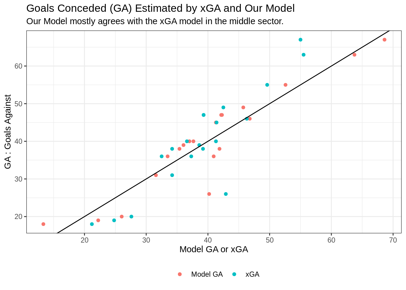 Our Model GA mostly aligns with that of the xGA estimation. Our model’s points (red) are slightly more optimized around the perfect model line (xGA = GA) especially at the extremities where this is more discrepancy between our model’s points and the xGA points.