30 Neural Network Ploting with BP Algorithm and without Algorithm
Jing Wang and Peilin Jing
30.1 Explnation of our community contribution:
30.1.1 Since we are learning data science as well as data visualization this semester, we get very interested in the data visualization in machine learning, and decide to do a tutorial for the Network plotting, which generally for the network visualization and bp neural network plotting.
30.1.2 We learned a lot from the project, including the neural networks we never lerned before, the basic network plotting, and how to scale the data for better visualization. Also, there are a few things we want to improve for next time. We would like to visualize more complex neural network algorithm, and would like to learn more about the network plotting packages including ggraph and ggnetwork.
30.2 The Back Propagation (bp) Neural Networks algorithm
BP (Back Propagation) neural network was proposed by scientists headed by Rumelhart and McCelland in 1986. It is a multi-layer feed-forward network trained by error Back Propagation algorithm. It is one of the most widely used neural network models at present. BP network can learn and store a large number of input-output mode mappings without revealing the mathematical equations describing the mappings in advance. Its learning rule is to use the fastest descent method, through back propagation to constantly adjust the weight and threshold of the network, so as to minimize the sum of squares of error of the network. The topology of BP neural network model includes input layer, hide layer and output layer. It can effectively decrease data dimensionality. To do this, we need to pass the data through the “bottleneck” with lower dimension than source data.
There are already many packages for bp neural networks in the R language, such as NNET, AMORE and Neuralnet.
Nnet provides the most common feed-forward and back-propagation neural network algorithm.
The AMORE package takes this one step further by providing richer control parameters and adding multiple hidden layers.
The Neuralnet package is improved by providing elastic backpropagation algorithms and more forms of activation functions.
The RSNNS package not only contains the bp algorithm but also other types of algorithm, such as DDA and etc.
Backpropagation neural networks can be very helpful whem we want to compress and visuallized multi_dimensional data, and it is more clear than some other well-known methods.
(https://link.springer.com/chapter/10.1007/978-3-642-30223-7_87; https://rpubs.com/alexv71/237757)
30.2.1 NNET
Feed-Forward Neural Networks and Multinomial Log-Linear Models
nnet uses the C code for BFGS from optim (converted earlier from Pascal) directly instead of calling optim from R. This may be what allows it to be faster, but limits the optimization to the single method. nnet is only beaten by the Extreme Learning Machine (ELM) algorithms in terms of speed. However, there is a larger variation when using nnet. We believe the different default starting values are the cause of this. For instance, nnet uses a range of initial random weights of 0.7 In spite of these results, the real reason most authors or users are likely to choose nnet is because it is included in the distributed base R and is even mentioned as the very first package in CRAN’s task view for machine learning.
(https://cran.r-project.org/web/packages/nnet/nnet.pdf)
30.2.1.1 Usage
nnet(x, …)
S3 method for formula
nnet(formula, data, weights, …,

subset, na.action, contrasts = NULL)
S3 method for default
nnet(x, y, weights, size, Wts, mask,

linout = FALSE, entropy = FALSE, softmax = FALSE,

censored = FALSE, skip = FALSE, rang = 0.7, decay = 0,

maxit = 100, Hess = FALSE, trace = TRUE, MaxNWts = 1000,

abstol = 1.0e-4, reltol = 1.0e-8, …)
30.2.1.2 Arguments
formula: A formula of the form class ~ x1 + x2 + …
x: matrix or data frame of x values for examples.
y: matrix or data frame of target values for examples.
weights: (case) weights for each example – if missing defaults to 1.
size: number of units in the hidden layer. Can be zero if there are skip-layer units.
data: Data frame from which variables specified in formula are preferentially to be taken.
subset: An index vector specifying the cases to be used in the training sample. (NOTE: If given, this argument must be named.)
na.action: A function to specify the action to be taken if NAs are found. The default action is for the procedure to fail. An alternative is na.omit, which leads to rejection of cases with missing values on any required variable. (NOTE: If given, this argument must be named.)
contrasts: a list of contrasts to be used for some or all of the factors appearing as variables in the model formula.
Wts: initial parameter vector. If missing chosen at random.
mask: logical vector indicating which parameters should be optimized (default all).
linout: switch for linear output units. Default logistic output units.
entropy: switch for entropy (= maximum conditional likelihood) fitting. Default by least-squares.
softmax: switch for softmax (log-linear model) and maximum conditional likelihood fitting. linout, entropy, softmax and censored are mutually exclusive.
censored: A variant on softmax, in which non-zero targets mean possible classes. Thus for softmax a row of (0, 1, 1) means one example each of classes 2 and 3, but for censored it means one example whose class is only known to be 2 or 3.
skip: switch to add skip-layer connections from input to output.
rang: Initial random weights on [-rang, rang]. Value about 0.5 unless the inputs are large, in which case it should be chosen so that rang * max(|x|) is about 1.
decay: parameter for weight decay. Default 0.
maxit: maximum number of iterations. Default 100.
Hess: If true, the Hessian of the measure of fit at the best set of weights found is returned as component Hessian.
trace: switch for tracing optimization. Default TRUE.
MaxNWts: The maximum allowable number of weights. There is no intrinsic limit in the code, but increasing MaxNWts will probably allow fits that are very slow and time-consuming.
abstol: Stop if the fit criterion falls below abstol, indicating an essentially perfect fit.
reltol: Stop if the optimizer is unable to reduce the fit criterion by a factor of at least 1 - reltol.
…
arguments passed to or from other methods.
#load package and data
# install.packages("DMwR2")
library(lattice)
library(grid)
library(DMwR2)
library(nnet)
data(algae)

#drop NAs
algae <- algae[-manyNAs(algae), ]
clean.algae <- knnImputation(algae[,1:12],k=10)

#approaching the value of NAs by finding the median of K neigbors
algae<-knnImputation(algae,k=10,meth='median')

# standardized data
norm.data <- scale(clean.algae[,4:12])

#use nnet to fit the model
nn <- nnet(a1~., norm.data, size = 10, decay = 0.01,
 maxit = 1000, linout = T, trace = F)

#use the model above to make prediction
norm.preds <- predict(nn, norm.data)

#plot predict value and true value
plot(norm.preds~ scale(clean.algae$a1))
#calculate the error
(nmse2 <- mean((norm.preds-scale(clean.algae$a1))^2)/
mean((mean( scale(clean.algae$a1))- scale(clean.algae$a1))^2))
## [1] 0.1452598
#plot model
library(devtools)
source_url('https://gist.githubusercontent.com/Peque/41a9e20d6687f2f3108d/raw/85e14f3a292e126f1454864427e3a189c2fe33f3/nnet_plot_update.r')
plot.nnet(nn)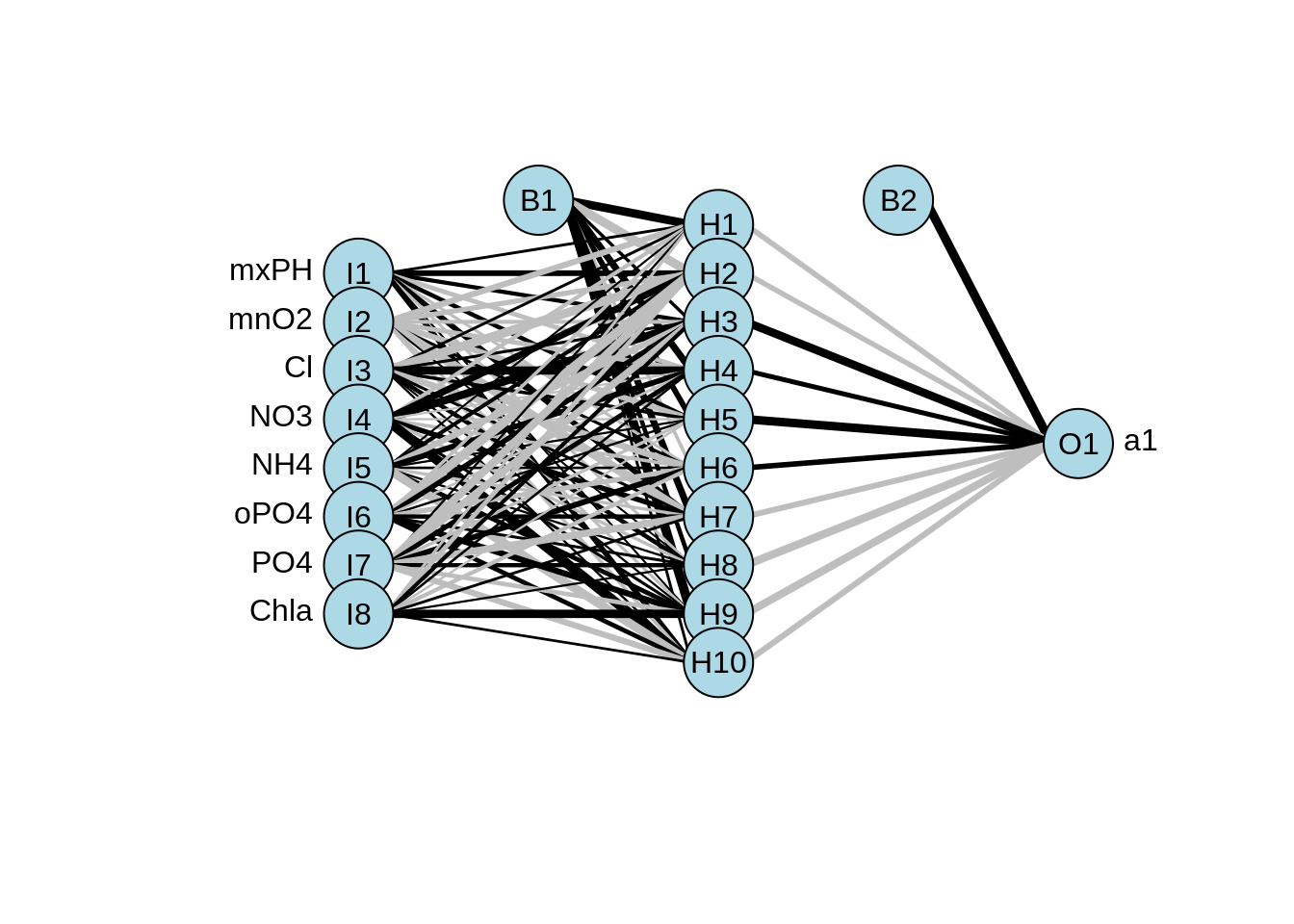
30.2.2 AMORE
AMORE is A MORE flexible neural network package, which was born to release the TAO robust neural network algorithem to the R users. It’s kind of out dated and hard to data visualization so that people generally will not use this one to do the bp neural network.
30.2.2.1 newff() Usage
newff(n.neurons, learning.rate.global, momentum.global,
error.criterium, Stao,hidden.layer, output.layer, method)
30.2.2.2 Arguments
n.neurons: Numeric vector containing the number of neurons of each layer. The first element of the vector is the number of input neurons, the last is the number of output neurons and the rest are the number of neuron of the different hidden layers.
learning.rate.global: Learning rate at which every neuron is trained.
momentum.global: Momentum for every neuron. Needed by several training methods
The mostly used arguments for newff() are listed above. For the further information, you can check on the cran website I posted below.
30.2.2.3 train() Usage
train(net, P, T, Pval=NULL, Tval=NULL, error.criterium="LMS",
report=TRUE,n.shows, show.step, Stao=NA,prob=NULL,n.threads=0L)
30.2.2.4 Arguments
net: Neural Network to train.
error.criterium: Criterium used to measure the goodness of fit:“LMS”, “LMLS”, “TAO”.
n.shows: Number of times to report (if report is TRUE). The total number of training epochs is n.shows times show.step.
show.step: Number of epochs to train non-stop until the training function is allow to report.
The mostly used arguments for train() are listed above. For the further information, you can check on the cran website I posted below.
(http://cran.nexr.com/web/packages/AMORE/AMORE.pdf)
#load package and data
library(remotes)
#install_version("AMORE", "0.2-11")
library(AMORE)

# Generate input data
P <- matrix(sample(seq(-1,1,length=1000),1000,replace=FALSE),ncol=1)

# Generate output data
target <- P^2

# Generate 2 hidden layers
net <- newff(n.neurons=c(1,3,2,1),
             learning.rate.global = 1e-2, momentum.global = 0.5)

# Train the neutral network
result <- train(net,P,target,error.criterium = "LMS", report = TRUE,
                show.step = 100,n.shows = 5)
## index.show: 1 LMS 0.0894144335797345
## index.show: 2 LMS 0.0893664649835284
## index.show: 3 LMS 0.0886648893419836
## index.show: 4 LMS 2.87892981034031e-05
## index.show: 5 LMS 2.130723629117e-05
# Predict for the result
y <- sim(result$net,P)
plot(P,y,col="blue",pch="+")
points(P,target,col="red",pch="x")
30.2.3 Neuralnet
This is a package that train the neural networks using back propagation,resilient back propagation with or without wright backtracking or the modified globally convergent. It alloes flexible settings through custom_choice of error and activation function. Furthermore, the calculation of generalized weights is imlemented. This one is generally used by many people, and is one of the most popular package for bp neural network.
30.2.3.1 neuralnet() Usage
neuralnet(formula, data, hidden = 1, threshold = 0.01,
 stepmax = 1e+05, rep = 1, startweights = NULL,
 learningrate.limit = NULL, learningrate.factor = list(minus = 0.5,
 plus = 1.2), learningrate = NULL, lifesign = "none",
 lifesign.step = 1000, algorithm = "rprop+", err.fct = "sse",
 act.fct = "logistic", linear.output = TRUE, exclude = NULL,
 constant.weights = NULL, likelihood = FALSE)
30.2.3.2 Arguments
formula: a symbolic description of the model to be fitted.
data: a data frame containing the variables specified in formula.
hidden: a vector of integers specifying the number of hidden neurons (vertices) in each layer.
threshold: a numeric value specifying the threshold for the partial derivatives of the error function as stopping criteria.
etc.
The mostly used arguments for neuralnet() are listed above. For the futher information, you can check on the cran website I posted below.
30.2.3.4 Arguments
x: an object of class nn.
covariate: a dataframe or matrix containing the variables that had been used to train the neural network.
rep: an integer indicating the neural network’s repetition which should be used.
(https://cran.r-project.org/web/packages/neuralnet/neuralnet.pdf)
#load package and data
# install.packages("neuralnet")
library(grid)
library(MASS)
library(neuralnet)

# Generate 50 data from 0 to 100 and turn it into input and output
traininginput <- as.data.frame(runif(50,min=0,max=100))
trainingoutput <- sqrt(traininginput)

# Combine input and output
trainingdata <- cbind(traininginput,trainingoutput)
colnames(trainingdata) <- c("Input", "Output")

# Train 10 hiddens for neural network
net.sqrt <- neuralnet(Output ~ Input, trainingdata, hidden=10,threshold=0.001)
summary(net.sqrt)
## Length Class Mode
## call 5 -none- call
## response 50 -none- numeric
## covariate 50 -none- numeric
## model.list 2 -none- list
## err.fct 1 -none- function
## act.fct 1 -none- function
## linear.output 1 -none- logical
## data 2 data.frame list
## exclude 0 -none- NULL
## net.result 1 -none- list
## weights 1 -none- list
## generalized.weights 1 -none- list
## startweights 1 -none- list
## result.matrix 34 -none- numeric
# Plot the neural network
plot(net.sqrt)

# Compute for the neutons
testdata <- as.data.frame((1:10)^2)
result <- compute(net.sqrt,testdata)
ls(result)
## [1] "net.result" "neurons"
print(result$net.result)## [,1]
## [1,] 1.001483
## [2,] 1.967301
## [3,] 3.009390
## [4,] 3.998934
## [5,] 5.002556
## [6,] 5.999033
## [7,] 6.999842
## [8,] 8.000364
## [9,] 8.999183
## [10,] 9.99497930.2.4 RSNSS
RSNSS is a new package for neural network, and it’s originally ceom for the SNNS library which wraps the SNNS functionality to make it available in R. Also, RSNSS expand the functionality and flexibility of SNNS which it contains more algorithms and topologies.
(https://cran.r-project.org/web/packages/RSNNS/RSNNS.pdf; https://rdrr.io/cran/RSNNS/man/mlp.html)
30.2.4.2 Arguments
y: inputs
method: “WTA” or “402040”
l: lower bound, e.g. in 402040: l=0.4 h upper bound, e.g. in 402040: h=0.6
#load package and data

# install.packages("RSNNS")
library(Rcpp)
library(RSNNS)

#load data
data(iris)

#use sample function to get random sample data set
 iris <- iris[sample(1:nrow(iris),length(1:nrow(iris))),1:ncol(iris)]

#define net input
 irisValues <- iris[,1:4]

#define net output, and transform the data format
 irisTargets <- decodeClassLabels(iris[,5])

#select training set and testing set
 iris <- splitForTrainingAndTest(irisValues, irisTargets, ratio=0.15)

#standardized data
 iris <- normTrainingAndTestSet(iris)

#use mlp to do the neural network algorithm (feed-forward)
model <- mlp(iris$inputsTrain, iris$targetsTrain, size=5, learnFuncParams=c(0.1), maxit=50, inputsTest=iris$inputsTest, targetsTest=iris$targetsTest)
summary(model)
## SNNS network definition file V1.4-3D
## generated at Tue Apr 12 21:44:45 2022
##
## network name : RSNNS_untitled
## source files :
## no. of units : 12
## no. of connections : 35
## no. of unit types : 0
## no. of site types : 0
##
##
## learning function : Std_Backpropagation
## update function : Topological_Order
##
##
## unit default section :
##
## act | bias | st | subnet | layer | act func | out func
## ---------|----------|----|--------|-------|--------------|-------------
## 0.00000 | 0.00000 | i | 0 | 1 | Act_Logistic | Out_Identity
## ---------|----------|----|--------|-------|--------------|-------------
##
##
## unit definition section :
##
## no. | typeName | unitName | act | bias | st | position | act func | out func | sites
## ----|----------|-------------------|----------|----------|----|----------|--------------|----------|-------
## 1 | | Input_1 | -0.29143 | 0.13084 | i | 1,0,0 | Act_Identity | |
## 2 | | Input_2 | -0.13387 | -0.00879 | i | 2,0,0 | Act_Identity | |
## 3 | | Input_3 | 0.19442 | -0.29257 | i | 3,0,0 | Act_Identity | |
## 4 | | Input_4 | 0.11948 | 0.00347 | i | 4,0,0 | Act_Identity | |
## 5 | | Hidden_2_1 | 0.83784 | 1.33418 | h | 1,2,0 |||
## 6 | | Hidden_2_2 | 0.22736 | -0.92067 | h | 2,2,0 |||
## 7 | | Hidden_2_3 | 0.12808 | -2.82738 | h | 3,2,0 |||
## 8 | | Hidden_2_4 | 0.39944 | 0.06052 | h | 4,2,0 |||
## 9 | | Hidden_2_5 | 0.31358 | -1.16370 | h | 5,2,0 |||
## 10 | | Output_setosa | 0.11700 | -0.60774 | o | 1,4,0 |||
## 11 | | Output_versicolor | 0.68134 | 0.50483 | o | 2,4,0 |||
## 12 | | Output_virginica | 0.07557 | -2.22674 | o | 3,4,0 |||
## ----|----------|-------------------|----------|----------|----|----------|--------------|----------|-------
##
##
## connection definition section :
##
## target | site | source:weight
## -------|------|---------------------------------------------------------------------------------------------------------------------
## 5 | | 4: 1.23525, 3: 1.32506, 2:-1.28824, 1: 0.92506
## 6 | | 4:-0.21415, 3:-1.29071, 2: 1.66811, 1:-0.67684
## 7 | | 4: 2.98342, 3: 2.10284, 2:-0.21317, 1:-0.39641
## 8 | | 4:-1.36627, 3:-1.16256, 2: 0.79454, 1:-0.09370
## 9 | | 4: 1.51683, 3: 1.03424, 2:-0.12963, 1: 0.06655
## 10 | | 9:-2.10872, 8: 2.42271, 7:-1.11247, 6: 1.36118, 5:-2.25204
## 11 | | 9:-0.89046, 8:-0.96601, 7:-3.94641, 6:-1.99330, 5: 2.24251
## 12 | | 9: 1.75366, 8:-3.31889, 7: 3.03418, 6:-0.56827, 5: 0.28522
## -------|------|---------------------------------------------------------------------------------------------------------------------
#use the model above to make prediction
par(mfrow=c(2,2))
plotIterativeError(model)
predictions <- predict(model,iris$inputsTest)
plotRegressionError(predictions[,2], iris$targetsTest[,2])

# Generate confusion matrix and plot ROC curve
confusionMatrix(iris$targetsTrain,fitted.values(model))
## predictions
## targets 1 2 3
## 1 43 0 0
## 2 0 37 3
## 3 0 1 43
confusionMatrix(iris$targetsTest,predictions)## predictions
## targets 1 2 3
## 1 7 0 0
## 2 0 10 0
## 3 0 0 6
plotROC(fitted.values(model)[,2], iris$targetsTrain[,2])
plotROC(predictions[,2], iris$targetsTest[,2])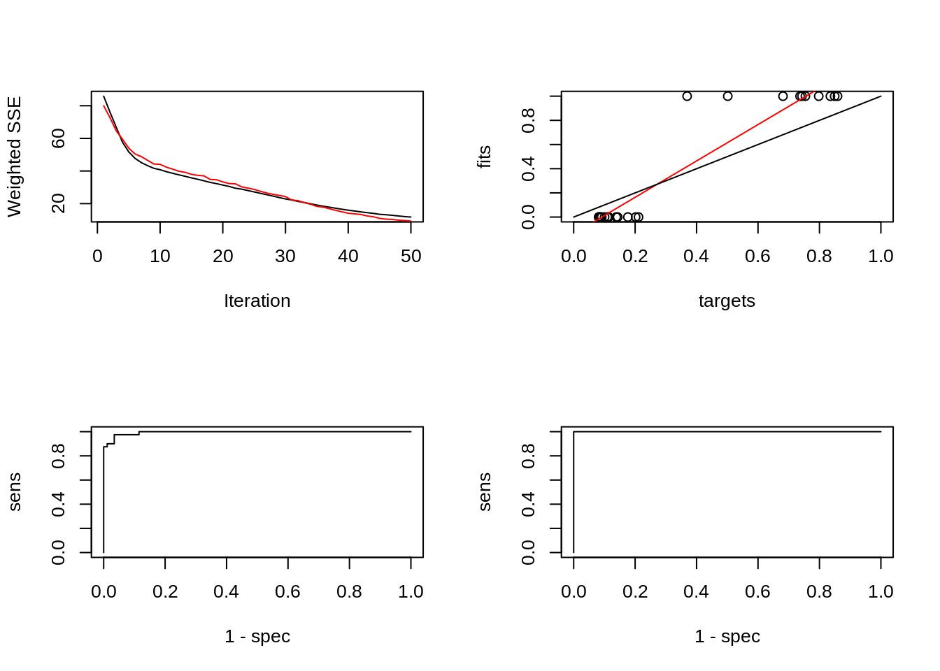
30.3 General plotting for Neural network
Network visualization allows administrators to quickly and intuitively understand a lot of information about the state of the network at a glance. If we are not sure about the algorithm, it’s better for us to visualize the network for our data. From the network visualization, we would like to find the key actors and links, the relationship strength, the structural properties and diffusion patterns, etc.
We would like to introduce two basic package for network visualizetion which are network and igraph. network can represent a range of relational data types, and supports arbitrary vertex/edge/graph attributes. igraph can handle large graphs very well and provides functions for generating random and regular graphs, graph visualization, centrality methods and much more.
(https://www.auvik.com/franklyit/blog/what-is-network-visualization/; https://kateto.net/network-visualization; https://cran.r-project.org/web/packages/igraph/igraph.pdf; https://cran.r-project.org/web/packages/network/network.pdf)
30.3.1 network
30.3.1.1 Usage
add.edge( x,
  tail,
  head,
  names.eval = NULL,
  vals.eval = NULL,
  edge.check = FALSE,
  ...
)
add.edges(x, tail, head, names.eval = NULL, vals.eval = NULL, ...)
30.3.1.2 Arguments
x: an object of class network
tail: for add.edge, a vector of vertex IDs reflecting the tail set for the edge to be added; for add.edges, a list of such vectors
head: for add.edge, a vector of vertex IDs reflecting the head set for the edge to be added; for add.edges, a list of such vectors
names.eval: for add.edge, an optional list of names for edge attributes; for add.edges, a list of length equal to the number of edges, with each element containing a list of names for the attributes of the corresponding edge
vals.eval: for add.edge, an optional list of edge attribute values (matching names.eval); for add.edges, a list of such lists
edge.check: logical; should we perform (computationally expensive) tests to check for the legality of submitted edges?
… additional arguments
set.seed(110)
library(network)
par(mfrow = c(2, 3))
# generate a three dots graph
net <- network.initialize(3)
plot(net,vertex.cex=10)
# add one edge
add.edge(net,2,3)
plot(net,vertex.cex=10, displaylabels=T)
# add two more dots
add.vertices(net,2)
plot(net,vertex.cex=10, displaylabels=T)
# generate a 5*12 dataframe
df <- matrix(rnorm(60),5)
# use covariance matrix to generate network
dfcor <- cor(df)
# remove the low correlation
dfcor[dfcor<0.5] <- 0
netcor <- as.network(dfcor,matrix.type = 'adjacency')
plot(netcor)
# add property to dots and edges
set.vertex.attribute(netcor, "class", length(netcor$val):1)
set.edge.attribute(netcor,"color",length(netcor$mel):1)
# more visual
plot(netcor,vertex.cex=5,vertex.col=get.vertex.attribute(netcor,"class"),edge.col=get.edge.attribute(netcor,'color'))
30.3.2 igraph
30.3.2.2 Arguments
e1: First argument, probably an igraph graph.
e2: Second argument.
set.seed(110)
library(igraph)
par(mfrow = c(2, 2))
# generate a three dots graph
net <- graph.empty(n=3, directed=TRUE)
plot(net)
# add two edges
new_edges <- c(1,3, 2,3)
net <- add.edges(net, new_edges)
plot(net)
# add two more dots
net <- add.vertices(net, 2)
plot(net)
# generate a 5*12 dataframe
df <- matrix(rnorm(60),5)
# use covariance matrix to generate network
dfcor <- cor(df)
# remove the low correlation
dfcor[dfcor<0.5] <- 0
net <- graph.adjacency(dfcor,weighted=TRUE,diag=FALSE)
plot(net)