41 Basic time series analysis and prediction
Dexin Sun
This is a tutorial for time series and prediction. The process of building a time series model and how to do the analysis will be covered.
41.1 Motivation
Time series analysis is a method to show the relationship between a variable and time. We usually use Yt as the value based on time t. The main purpose of time series analysis is to do the prediction based on historical data. This tutorial will focus on how to build a time series model and do the prediction.
41.2 Data input
We use the dataset in R call “sunspot.month”. This is a monthly numbers of sunspots, as from the World Data Center.
41.3 Time series plot
First, we could use “plot.ts()” to show the time series plot, this is a direct way to show the relationship between a variable and time.
Most of time series model could be divide into 3 components: stationary series, trend, seasonal variation. Definition of Stationary Series is that joint probability distributions do not change with time or expectation and variance do not change with time, meaning that statistical value fluctuates up and down a constant and the fluctuation range is bounded.
For example, in the plot below, we could find that it is a model with seasonality but the trend is not obvious. And stationary series is what we could choose a model to fit.
The autocorrelation coefficient ACF characterizes the correlation coefficient between yt and the lag k-order Y(t-k), and the partial autocorrelation coefficient PACF characterizes the removal of the Y(t-1), Y(t-2) equivalent pair Y(t-k) after the impact of the correlation coefficient. ACF and PACF could show the stationary of model. Both of them are shown, as follows:
plot.ts(sunspot.month)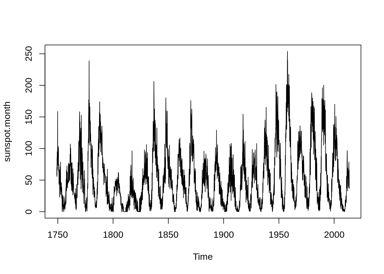
acf(sunspot.month)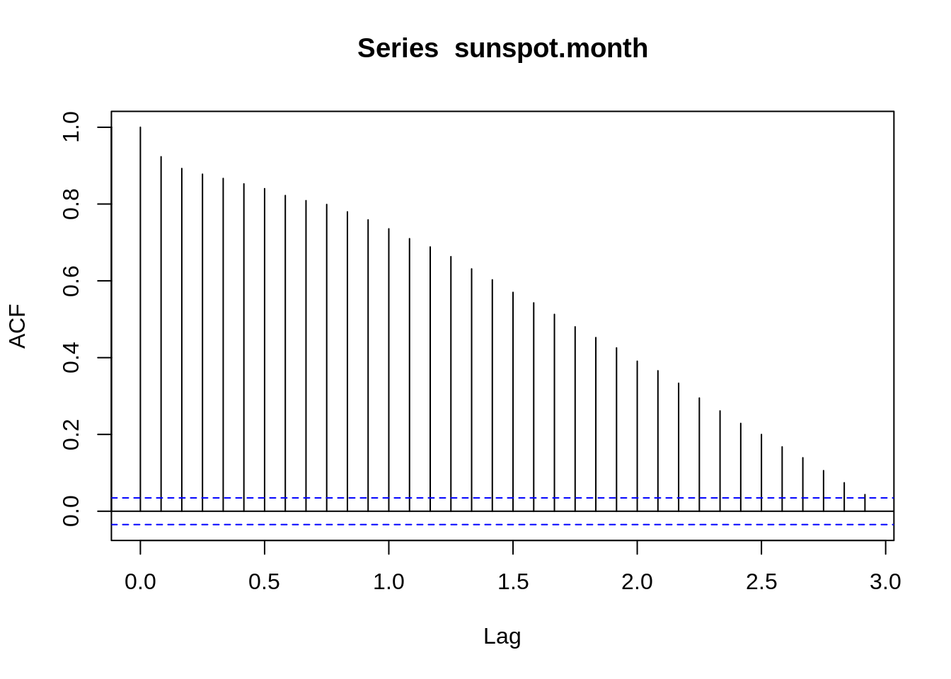
pacf(sunspot.month)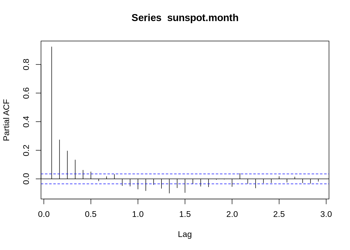
To get stationary series, we need to remove trend and seasonal variation. There are two common ways: Smoothing and differencing. Smoothing is a way to get the function of trend and seasonality, which is hard to find. Differencing is what we will focus in this tutorial.
41.4 Differencing
We could use “adf.test()” to verify whether we need to differencing. “ndiffs()” could show the difference order.
adf.test(sunspot.month)##
## Augmented Dickey-Fuller Test
##
## data: sunspot.month
## Dickey-Fuller = -7.0245, Lag order = 14, p-value = 0.01
## alternative hypothesis: stationary
ndiffs(sunspot.month)## [1] 1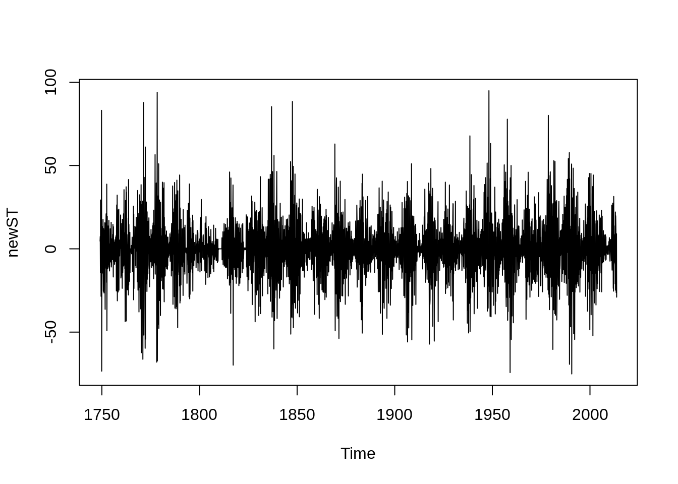
acf(newST)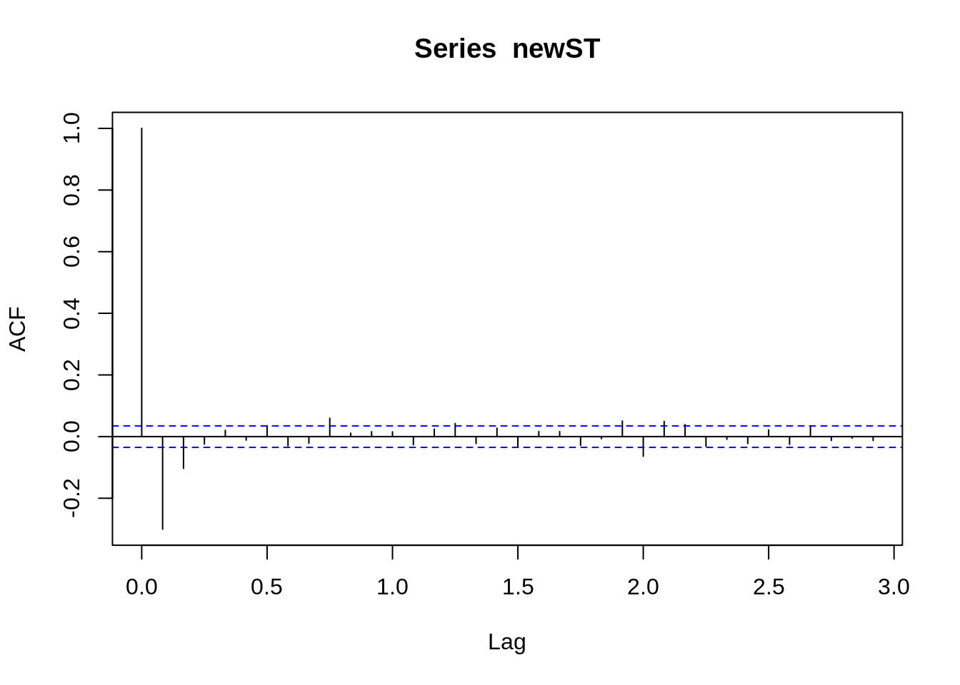
pacf(newST)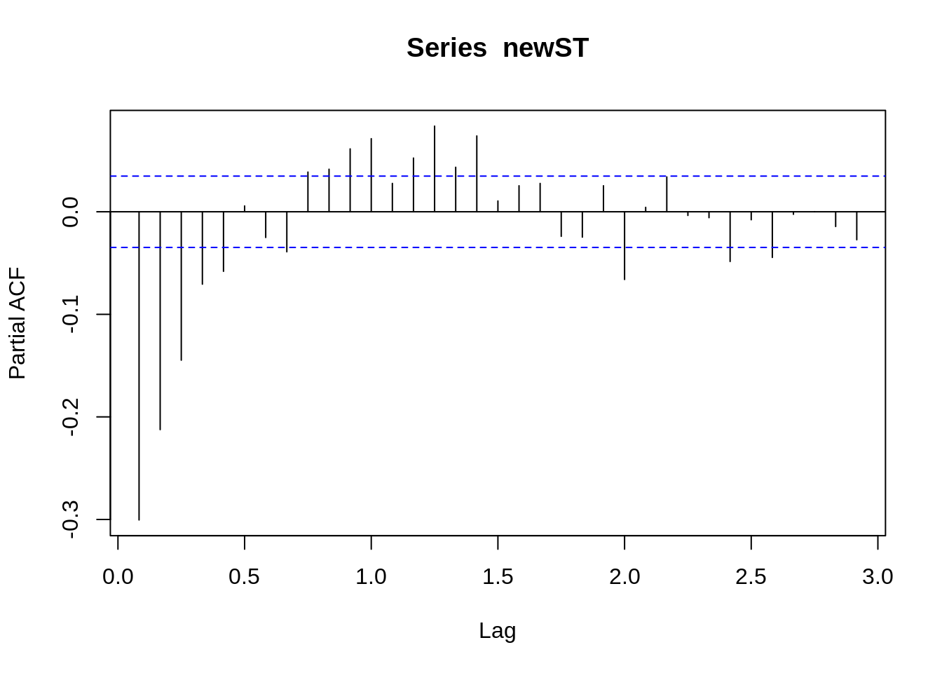
41.5 Stationary series model
There are three common stationary series models:
AR(p): Autoregression. The evolving variable of interest is regressed on its own lagged values.
MA(q): Moving Average. The regression error is actually a linear combination of error terms whose values occurred contemporaneously and at various times in the past.
ARMA(p,q): Autoregressive moving average. AR+MA
The model without differencing is ARIMA(p,d,q) model, where:
I: Integrated. The data values have been replaced with the difference between their values and the previous values.
p: The order (number of time lags) of the autoregressive model
d:The degree of differencing
q: The order of the moving-average model
From the figure above, it can be seen that the sequence after the differencing becomes a stationary sequence. And the autocorrelation graph shows that the autocorrelation coefficient quickly decreases to 0 after lagging 1 order, which further shows that the series is stable. According to the figure below, the sequence after the differencing applies to ARIMA(5,1,2). And ARIMA(5,1,2) could be the beginning parameter, and based on the beginning parameter we could do some small adjustment to gain the best model.
##
## Call:
## arima(x = sunspot.month, order = c(5, 1, 2), method = "ML")
##
## Coefficients:
##           ar1      ar2      ar3      ar4      ar5     ma1      ma2
##       -0.5212  -0.2156  -0.1722  -0.0812  -0.0498  0.1113  -0.1250
## s.e.   0.2677   0.2113   0.1044   0.0699   0.0359  0.2677   0.1908
##
## sigma^2 estimated as 252.1: log likelihood = -13287.92, aic = 26591.84##
## Call:
## arima(x = sunspot.month, order = c(4, 1, 2), method = "ML")
##
## Coefficients:
## ar1 ar2 ar3 ar4 ma1 ma2
## -0.197 -0.0578 -0.0672 -0.0101 -0.213 -0.1488
## s.e. NaN NaN 0.0209 0.0264 NaN NaN
##
## sigma^2 estimated as 252.3: log likelihood = -13289.34, aic = 26592.67##
## Call:
## arima(x = sunspot.month, order = c(3, 1, 2), method = "ML")
##
## Coefficients:
## ar1 ar2 ar3 ma1 ma2
## -0.1889 -0.0398 -0.0582 -0.2208 -0.1636
## s.e. NaN NaN NaN NaN NaN
##
## sigma^2 estimated as 252.3: log likelihood = -13289.41, aic = 26590.82##
## Call:
## arima(x = sunspot.month, order = c(2, 1, 2), method = "ML")
##
## Coefficients:
## ar1 ar2 ma1 ma2
## 1.3304 -0.3805 -1.7581 0.7979
## s.e. 0.0289 0.0272 0.0198 0.0186
##
## sigma^2 estimated as 246.3: log likelihood = -13251.08, aic = 26512.17##
## Call:
## arima(x = sunspot.month, order = c(1, 1, 2), method = "ML")
##
## Coefficients:
## ar1 ma1 ma2
## -0.0099 -0.3995 -0.1246
## s.e. 0.1104 0.1089 0.0538
##
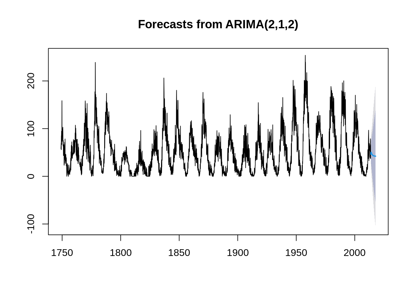
## sigma^2 estimated as 252.7: log likelihood = -13291.64, aic = 26591.28Compared all AIC value above, we could find that ARIMA(2,1,2) has the smallest model. Therefore, ARIMA(2,1,2) would be the fittest model.
Or “auto.arima” could be use to find the fittest model, which is a easier method:
auto.arima(sunspot.month)## Series: sunspot.month
## ARIMA(2,1,2)
##
## Coefficients:
## ar1 ar2 ma1 ma2
## 1.3307 -0.3807 -1.7582 0.7979
## s.e. 0.0289 0.0272 0.0198 0.0186
##
## sigma^2 = 246.6: log likelihood = -13251.08
## AIC=26512.17 AICc=26512.19 BIC=26542.4841.6 Testing
TSmodel <- auto.arima(sunspot.month)
shapiro.test(TSmodel$residuals)
##
## Shapiro-Wilk normality test
##
## data: TSmodel$residuals
## W = 0.96263, p-value < 2.2e-16
Box.test(TSmodel$residuals)##
## Box-Pierce test
##
## data: TSmodel$residuals
## X-squared = 0.16254, df = 1, p-value = 0.6868The parameter test includes two tests: the significance test of the parameters and the normality and irrelevance test of the residuals. We could use “shapiro.test()” to check the normality of residuals and “Box.test()” to check the randomness of residuals. Since p-value of normality test is smaller than 0.05, stationary series is not a normal distribution.