97 ANOVA tutorial
Xinrui Bai and Zewen Shi
The main motivation for this community contribution project is to provide a tutorial of a few useful visualization tools in the process of the analysis of variances, a common topic that statisticians deal with on a daily basis. This project will walk users through such tools of visualization and how they would be a complement to concrete test results by making them understandable even by audiences with little training in statistics. In the first part, the background for a typical problem of our choice will be provided and manipulations of the data will be carried out to obtain a model of best fit for later use. In the second part, diagnosis using visualization tools will be conducted and results will be analyzed.
#.libPaths("C:/Rpackage")
library(car)
library(MASS)
library(tidyverse)
library(glmnet)
library(ggplot2)
library(ggpubr)
library(tidyverse)
library(broom)
#library(AICcmodavg)
97.1 Part 1: Background and Preliminary Data Manipulation
Analysis of variance (ANOVA) is a collection of statistical models and their associated estimation procedures (such as the “variation” among and between groups) used to analyse the differences among means. ANOVA was developed by the statistician Ronald Fisher. ANOVA is based on the law of total variance, where the observed variance in a particular variable is partitioned into components attributable to different sources of variation. In its simplest form, ANOVA provides a statistical test of whether two or more population means are equal, and therefore generalizes the t-test beyond two means.(Wikipedia)
97.1.1 Step 1: taking a first look at the dataset:
crop.data <- read.csv("resources/anova_tutorial/cropdata.csv", header = TRUE, colClasses = c("factor", "factor", "factor", "numeric")) # if data is in the $home folder

summary(crop.data)
## density block fertilizer yield
## 1:48 1:24 1:32 Min. :175.4
## 2:48 2:24 2:32 1st Qu.:176.5
## 3:24 3:32 Median :177.1
## 4:24 Mean :177.0
## 3rd Qu.:177.4
## Max. :179.1Taking a first look at the data, we have observed multicollinearity in the dataset because VIF > 10. In a standard anova test, we test if any of the group means are significantly different from others by comparing variances. If the test fails, it means at least one group significant deviates from the overall mean.
97.1.2 Step 2: one-way anova
##             Df Sum Sq Mean Sq F value Pr(>F)
## fertilizer   2   6.07  3.0340   7.863  7e-04 ***
## Residuals   93  35.89  0.3859
## ---
## Signif. codes:  0 '***' 0.001 '**' 0.01 '*' 0.05 '.' 0.1 ' ' 1
This tests the null hypothesis, which states that samples in all groups are drawn from populations with the same mean values. To do this, two estimates are made of the population variance. These estimates rely on various assumptions (see below). The ANOVA produces an F-statistic, the ratio of the variance calculated among the means to the variance within the samples. If the group means are drawn from populations with the same mean values, the variance between the group means should be lower than the variance of the samples, following the central limit theorem. A higher ratio therefore implies that the samples were drawn from populations with different mean values. In this one-way ANOVA setup, we test if fertilizer type has a significant impact on the final crop yield. Since we received a p-value smaller than 0.001, there exists such impact.
97.1.3 Step 3:two-way data
#anova adjust for two independent variables
#start to generate the dataset for two x variables
anova2way <- aov(yield ~ fertilizer + density, data = crop.data)
summary(anova2way)
## Df Sum Sq Mean Sq F value Pr(>F)
## fertilizer 2 6.068 3.034 9.073 0.000253 ***
## density 1 5.122 5.122 15.316 0.000174 ***
## Residuals 92 30.765 0.334
## ---
## Signif. codes: 0 '***' 0.001 '**' 0.01 '*' 0.05 '.' 0.1 ' ' 1In statistics, the two-way analysis of variance (ANOVA) is an extension of the one-way ANOVA that examines the influence of two different categorical independent variables on one continuous dependent variable. The two-way ANOVA not only aims at assessing the main effect of each independent variable but also if there is any interaction between them. In this two-way ANOVA setup, adding planting density has reduced the residual variance and both variables appear to have a significant impact on the final crop yield since the p-values are small.
97.1.4 Step 4: adding interaction terms
#generate the anova for the data
anova_inter <- aov(yield ~ fertilizer*density, data = crop.data)
#display the results
summary(anova_inter)
## Df Sum Sq Mean Sq F value Pr(>F)
## fertilizer 2 6.068 3.034 9.001 0.000273 ***
## density 1 5.122 5.122 15.195 0.000186 ***
## fertilizer:density 2 0.428 0.214 0.635 0.532500
## Residuals 90 30.337 0.337
## ---
## Signif. codes: 0 '***' 0.001 '**' 0.01 '*' 0.05 '.' 0.1 ' ' 1In this step, we exploit if the interaction between the two variables has a significant impact on the variance, and the test results with a high p-value proved it did not.
97.1.5 Step 5: blocking variable
#generate the anova for the data
anova_block <- aov(yield ~ fertilizer + density + block, data = crop.data)
#display the results
summary(anova_block)
## Df Sum Sq Mean Sq F value Pr(>F)
## fertilizer 2 6.068 3.034 9.018 0.000269 ***
## density 1 5.122 5.122 15.224 0.000184 ***
## block 2 0.486 0.243 0.723 0.488329
## Residuals 90 30.278 0.336
## ---
## Signif. codes: 0 '***' 0.001 '**' 0.01 '*' 0.05 '.' 0.1 ' ' 1The intuition behind this step is that in many crop yield studies, treatments are applied within “blocks” in the field that may have some influence over the objectivity of the test. The effect of this difference was tested by adding a third term, and as shown on the test result, the block term was not statistically significant.
97.1.6 Step 6: obtaining the best-fitting model
#library(AICcmodavg)

#allanovas <- list(anovaoneway, anova2way, anova_inter, anova_block)
#allanovasnames <- c("one way Anova", "two way Anova", "Anova wtih interaction term", "Anova with a blocking term")

#aictab(allanovas, modnames = allanovasnames)
We plan to use the aictab() function from the AICcmodavg plackage to obtain the best-fitting model among the four different ANOVA models.This function creates a model selection table based on one of the following information criteria: AIC, AICc, QAIC, QAICc. The table ranks the models based on the selected information criteria and also provides delta AIC and Akaike weights. But due to some version and software issues. The codes won’t work so we just display the process here. However it can work days ago so we can display the results.
Since this step, we have exploited several measures to lock down potential combinations of variables to figure out what would be the best-fitting model for this dataset. We have finally chosen the two way model to be our best fitting model because it has the lowest AIC score. In the next part, we will run some diagnosis and tests on this model using both concrete tests and visualization tools.
97.2 Part 2: Visualization and Diagnosis
97.2.1 Step 1: homoskedasticity test
par(mfrow=c(1,1))

#ggplot2 for Q-Q plot
qqnorm(resid(anova2way));qqline(resid(anova2way), col = 2,lwd=2,lty=2)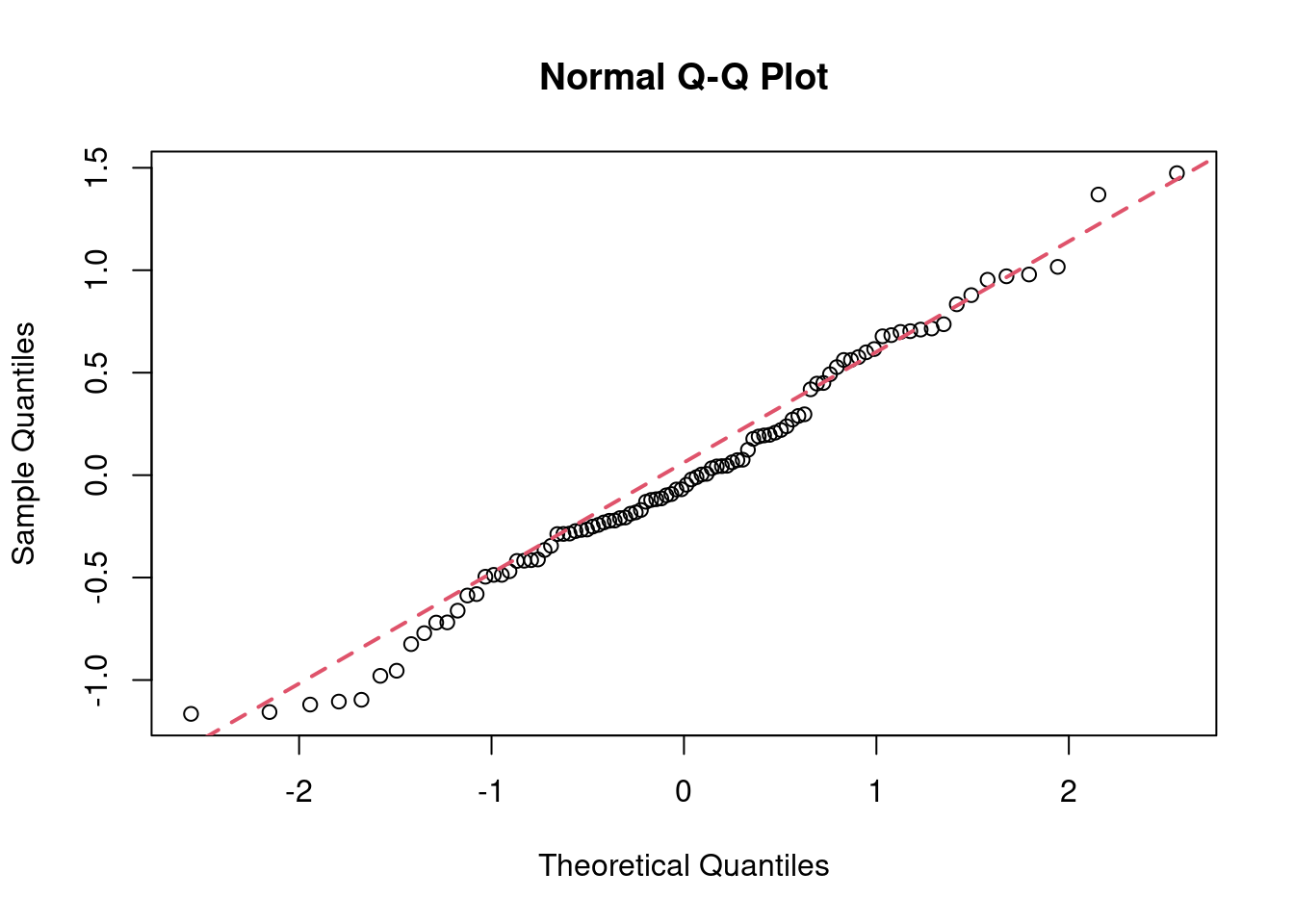
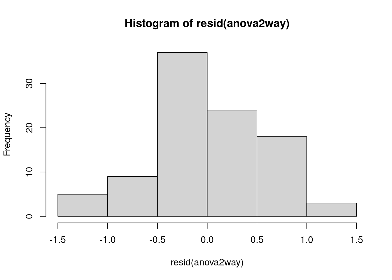
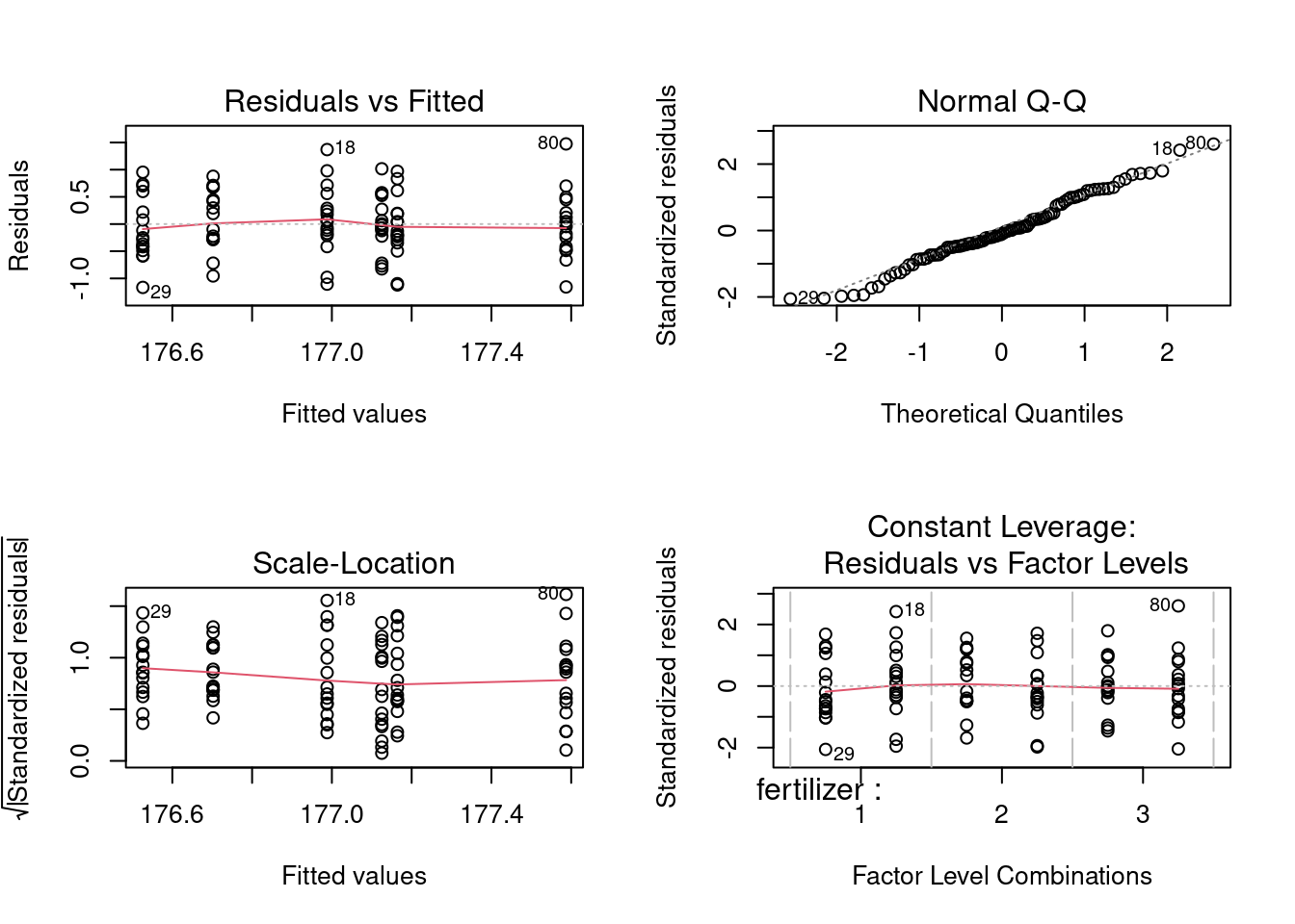
In this step, the normal Q-Q plot gives us visual clues on how much the dataset deviates from normal distribution, which is not much, as confirmed by the shaprp-ratio test with a p-value of 0.8836>0.05
While interpreting the first set of graphs, it is usually important to know the red line represents the mean of residuals and it should be horizontal and scattered around the value 0 or 1 for the normality assumption to hold, otherwise there exists significant outliers that have bigger than normal influence on the model, causing unneccessary bias.
For remedial measures we can use Box-Cox transformation, or fit Generalized Linear Model. We may also use nonparametric or robust procedures.
97.2.2 Step 2: parallelism test
#check for parallelism
#two-way anova
anova_inter<-aov(yield ~ fertilizer*density, data = crop.data)
summary(anova_inter)
## Df Sum Sq Mean Sq F value Pr(>F)
## fertilizer 2 6.068 3.034 9.001 0.000273 ***
## density 1 5.122 5.122 15.195 0.000186 ***
## fertilizer:density 2 0.428 0.214 0.635 0.532500
## Residuals 90 30.337 0.337
## ---
## Signif. codes: 0 '***' 0.001 '**' 0.01 '*' 0.05 '.' 0.1 ' ' 1Because the P-value=0.353 >0.05, we fail to reject H0. There is no significant interaction between birthweight and diet. There is no inference about the marginal mean differences must be performed.
Remedial Measures: when H0 is rejected that implies we don’t have parallelism, the relationship becomes much more complicated than we expect. The best way we should do is to just compare the group means at each value of x, like birth weight, individually.
97.2.3 Step 3: Unequal Variances test
#bartlett test on data
bartlett.test(x=crop.data$yield,g=crop.data$density)
##
## Bartlett test of homogeneity of variances
##
## data: crop.data$yield and crop.data$density
## Bartlett's K-squared = 0.16171, df = 1, p-value = 0.6876
#levene test on data
library(car)
leveneTest(y=crop.data$yield,group=as.factor(crop.data$density))
## Levene's Test for Homogeneity of Variance (center = median)
## Df F value Pr(>F)
## group 1 0.152 0.6975
## 94Bartlett’s test is sensitive to departures from normality. That is, if your samples come from non-normal distributions, then Bartlett’s test may simply be testing for non-normality. The Levene test is an alternative to the Bartlett test that is less sensitive to departures from normality.
Based on the Bartlett test, The p-value is 0.3, which is larger than 0.05. We fail to reject the null hypothesis, the constant variance assumption satisfies.
Based on the Levene’s test, The p-value is 0.38, which is larger than 0.05. We fail to reject the null hypothesis, the constant variance assumption satisfies.
Remedial Measures: we can use weighted Least Squares,transform Y and/or X, or fit Generalized Linear Mode to solve the problem.
97.2.4 Step 4: post-hoc test
tukeytest<-TukeyHSD(anova2way)

tukeytest
## Tukey multiple comparisons of means
## 95% family-wise confidence level
##
## Fit: aov(formula = yield ~ fertilizer + density, data = crop.data)
##
## $fertilizer
## diff lwr upr p adj
## 2-1 0.1761687 -0.16822506 0.5205625 0.4452958
## 3-1 0.5991256 0.25473179 0.9435194 0.0002219
## 3-2 0.4229568 0.07856306 0.7673506 0.0119381
##
## $density
## diff lwr upr p adj
## 2-1 0.461956 0.2275205 0.6963916 0.0001741In a scientific study, post hoc analysis (from Latin post hoc, “after this”) consists of statistical analyses that were specified after the data were seen. This typically creates a multiple testing problem because each potential analysis is effectively a statistical test. Multiple testing procedures are sometimes used to compensate, but that is often difficult or impossible to do precisely. Post hoc analysis that is conducted and interpreted without adequate consideration of this problem is sometimes called data dredging by critics because the statistical associations that it finds are often spurious.
ANOVA tests only gives information about whether group means significantly differ but not the numerical value of the differences. To get a more comprehensive results and find out how much they actually differ, we conduct a Tukey’s HSD post-hoc test. Based on the results, fertilizer types 2 and 3, fertilizer groups 1 and 3, and two levels of planting density have demonstrated statistically significant differences.
97.2.5 Step 5: visualized test results
tukey_plot<-aov(yield ~ fertilizer:density, data=crop.data)
tukey.plot<-TukeyHSD(tukey_plot)
plot(tukey.plot, las = 1,col = c("red", "blue", "green", "orange"))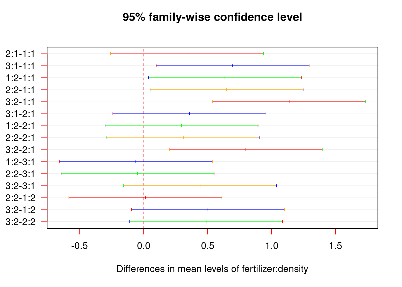
As shown on the graph, if the confidence interval does not include zero, it means the p-value for the difference is smaller than 0.05, as evidence of significant differences.
97.2.6 Step 6: creating a data frame with the group labels and more visualizations
yielddata <- crop.data %>%
  group_by(fertilizer, density) %>%
  summarise(
    yield = mean(yield)
  )


#mergeDay18_meanData, weight ~ birthweight + Diet


yielddata$group <- c("a","b","b","b","b","c")

yielddata
## # A tibble: 6 × 4
## # Groups: fertilizer [3]
## fertilizer density yield group
## <fct> <fct> <dbl> <chr>
## 1 1 1 176. a
## 2 1 2 177. b
## 3 2 1 177. b
## 4 2 2 177. b
## 5 3 1 177. b
## 6 3 2 178. c
ggplot(crop.data, aes(x = density, y = yield, group=density)) +
geom_boxplot() +
geom_jitter(shape = 15,
color = "steelblue",
position = position_jitter(0.21)) +
theme_classic()+
ggtitle("Boxplot between different density of the crop data")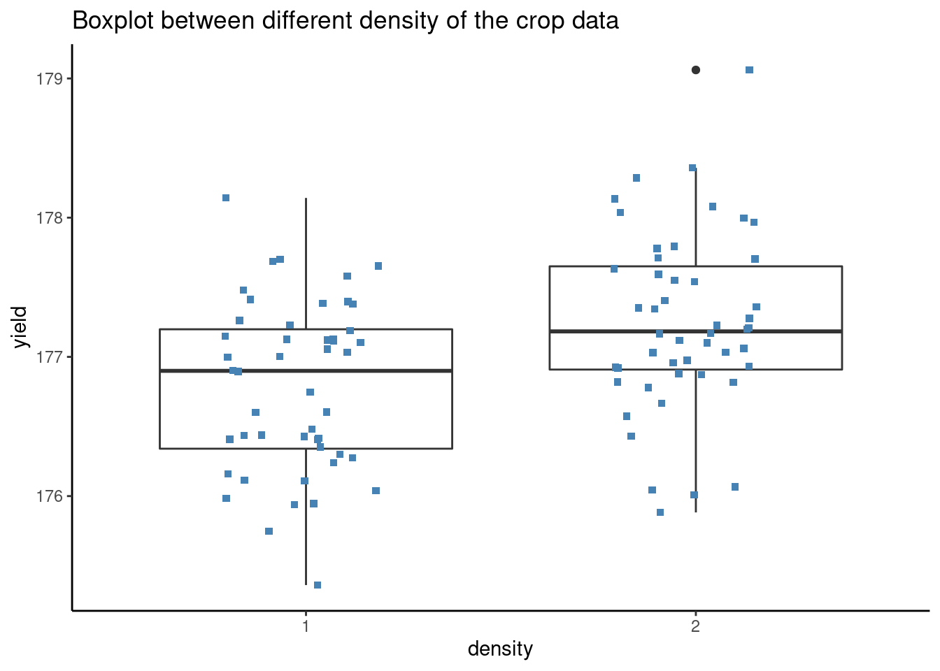 The group labels work as follows: A 1:1, C 3:2, B: other intermediate combinations.
Twoway <- ggplot(crop.data, aes(x = density, y = yield, group=fertilizer, fill=fertilizer),color='darkblue') +
  geom_point(cex = 1.5, pch = 1.0,position = position_jitter(w = 0.1, h = 0))+

  ggtitle("Two way plot of the crop data based on fertilizer")+
  scale_color_gradientn(colours = rainbow(5))
Twoway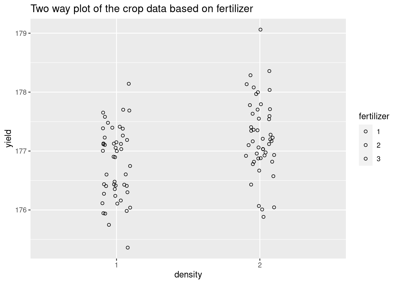
plot1<- Twoway +
  stat_summary(fun.data = 'mean_se', geom = 'errorbar', width = 0.2,color='blue') +
  stat_summary(fun.data = 'mean_se', geom = 'pointrange',color='red') +
  geom_point(data=yielddata, aes(x=density, y=yield, fill=density),color='green')+

  ggtitle("Two way plot of the crop data with means")
plot1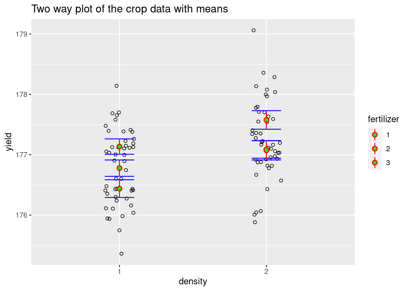
We have obtained a preliminary visualization but all the groups are stacked on top of each other, which makes it difficult to read. In the next step, we separate them.
plot2 <- Twoway +
  geom_text(data=yielddata, label=yielddata$group, vjust = -8, size = 5) +
  facet_wrap(~ fertilizer)+

  ggtitle("Two way plot of the crop data with full separation")

plot2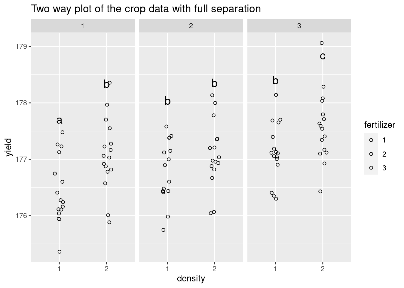
plot3 <- Twoway +
theme_classic2() +
labs(title = "Crop yield with different kinds of fertilizer and planting density",
x = "Planting density (0=low density, 1=high density)",
y = "Yield (bushels)")
plot3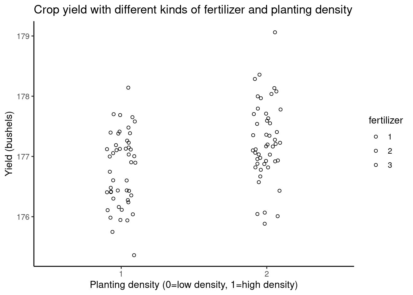 With added labels, the final visualization looks like this.
97.3 Part 3: Summary
In the first part, the background for a typical problem of our choice will be provided and manipulations of the data will be carried out to obtain a model of best fit for later use. In the second part, diagnosis using visualization tools will be conducted and results will be analyzed. However, we drifted away from the original purpose that specifically focused on visualization and decided to give a more step-by-step tutorial on how to conduct an ANOVA test with specific instructions, because it was our opinion that the ANOVA test is such an important topic in statistics and it is imperative that readers understand the statistical reasons behind every step and only then can they begin to interpret the visualization tools we employed. After working on this project, we have reinforced our understanding of how visualization and concrete mathematical tests work together to help statisticians make decisions to adjust their models or arrive at a certain conclusion.
Reference
ggplot2 colors : How to change colors automatically and manually?: http://www.sthda.com/english/wiki/ggplot2-colors-how-to-change-colors-automatically-and-manually ANOVA in R: A step-by-step guide, Published on March 6, 2020 by Rebecca Bevans. Revised on July 1, 2021.https://www.scribbr.com/statistics/one-way-anova/ Analysis of variance: https://en.wikipedia.org/wiki/Analysis_of_variance Stats and R:https://statsandr.com/blog/anova-in-r/