87 Tutorial on R Markdown

Anni Chen

87.1 R code chunks and inline R code

A code chunk is one of the main element of R Markdown where all R codes can be run in it. There are a lot of things you can do in a code chunk: you can produce text output, tables, or graphics. You have fine control over all these output via chunk options, which can be provided inside the curly braces (between {r and }). For example, you can choose hide text output via the chunk option results = ‘hide’, or set the figure height to 4 inches via fig.height = 4. Chunk options are separated by commas.

There are a large number of chunk options in knitr. Here listed some most commonly used options:

eval: Whether to evaluate a code chunk.
echo: Whether to echo the source code in the output document.
collapse: Whether to merge text output and source code into a single code block in the output. This is mostly cosmetic: collapse = TRUE makes the output more compact, since the R source code and its text output are displayed in a single output block. The default collapse = FALSE means R expressions and their text output are separated into different blocks.
warning, message, and error: Whether to show warnings, messages, and errors in the output document. Note that if you set error = FALSE, rmarkdown::render() will halt on error in a code chunk, and the error will be displayed in the R console. Similarly, when warning = FALSE or message = FALSE, these messages will be shown in the R console.
include: Whether to include anything from a code chunk in the output document. When include = FALSE, this whole code chunk is excluded in the output, but note that it will still be evaluated if eval = TRUE. When you are trying to set echo = FALSE, results = 'hide', warning = FALSE, and message = FALSE, chances are you simply mean a single option include = FALSE instead of suppressing different types of text output individually.
cache: Whether to enable caching. If caching is enabled, the same code chunk will not be evaluated the next time the document is compiled (if the code chunk was not modified), which can save you time. However, I want to honestly remind you of the two hard problems in computer science (via Phil Karlton): naming things, and cache invalidation. Caching can be handy but also tricky sometimes.
fig.width and fig.height: The (graphical device) size of R plots in inches. R plots in code chunks are first recorded via a graphical device in knitr, and then written out to files. You can also specify the two options together in a single chunk option fig.dim, e.g., fig.dim = c(6, 4) means fig.width = 6 and fig.height = 4.
out.width and out.height: The output size of R plots in the output document. These options may scale images. You can use percentages, e.g., out.width = '80%' means 80% of the page width.

Here taking Question 5 in HW1 as an example:

library(openintro)
library(ggplot2)
loans <- openintro::loans_full_schema
ggplot(loans,aes(loan_amount,fill=grade))+geom_histogram(binwidth = 2000,color='white')+ggtitle('Histogram of loan amount with different loan grade')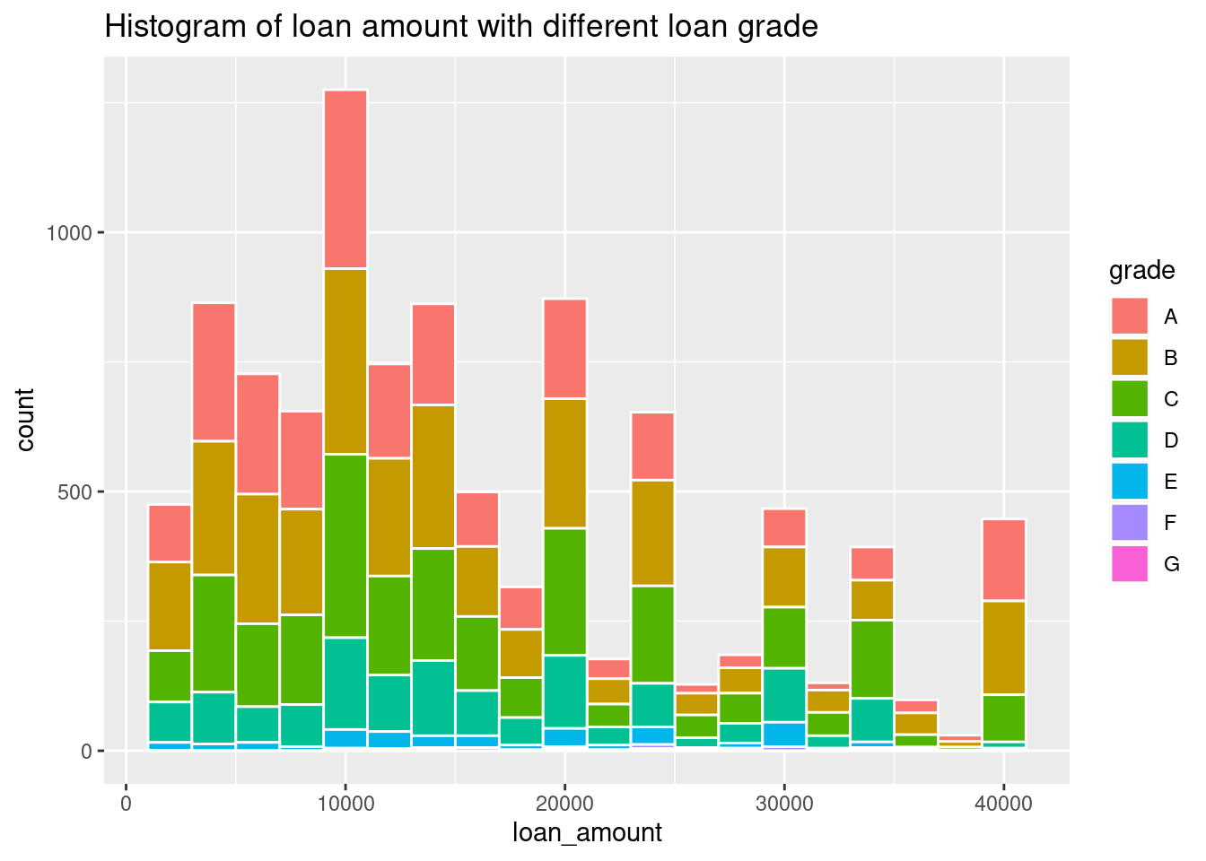

To only show the result as well as ignore the warning, we can customize the options:

warning=FALSE,error=FALSE,echo = FALSE, out.width = '50%'

87.2 Markdown syntax

The text in an R Markdown document is written with the Markdown syntax. Precisely speaking, it is Pandoc’s Markdown. There are many flavors of Markdown invented by different people, and Pandoc’s flavor is the most comprehensive one to our knowledge. You can find the full documentation of Pandoc’s Markdown at https://pandoc.org/MANUAL.html.

87.2.1 Inline information

Inline text will be italic if surrounded by underscores or asterisks, e.g., _text_ or *text*. Bold text is produced using a pair of double asterisks (**text**). A pair of tildes (~) turn text to a subscript (e.g., H~3~PO~4~ renders H3PO4). A pair of carets (^) produce a superscript (e.g., Cu^2+^ renders Cu²⁺).
To mark text as inline code, use a pair of backticks, e.g., code. To include n literal backticks, use at least n+1 backticks outside, e.g., you can use four backticks to preserve three backtick inside: ```code```, which is rendered as code.
Using HTML syntax to change Font: Data Visulization gives Data Visulization
Using HTML syntax to change font size: Data Visulization gives Data Visulization
Using HTML syntax to change font color: Data Visulization gives Data Visulization
Using HTML syntax to change background color: Data Visulization gives Data Visulization
Hyperlinks are created using the syntax [text](link), e.g., [RStudio](https://www.rstudio.com) will be like: RStudio.
The syntax for images is similar: just add an exclamation mark, e.g., ![alt text or image title](path/to/image). Here for example:![cute kitten](resources/Introduction_to_RMarkdown/cute_kitten.jpg)
Footnotes are put inside the square brackets after a caret ^[], e.g., ^[This is a footnote.]

87.2.2 Block-level elements

Section headers can be written after a number of pound signs, e.g.,

# First-level header

## Second-level header

### Third-level header

87.3 Second-level header

87.3.1 Third-level header

If you do not want a certain heading to be numbered, you can add {-} or {.unnumbered} after the heading, e.g.,# Preface {-}

Unordered list items start with *,-, or +, and you can nest one list within another list by indenting the sub-list, e.g.

- one item
- one item
- one item
    - one more item
    - one more item
    - one more item

and the output will be like:

one item
one item
one item
- one more item
- one more item
- one more item

Plain code blocks can be written after three or more backticks, and you can also indent the blocks by four spaces, e.g.,

```
This text is displayed verbatim / preformatted
```

Or indent by four spaces:

    This text is displayed verbatim / preformatted

In general, you’d better leave at least one empty line between adjacent but different elements, e.g., a header and a paragraph.

87.3.2 Math expressions

Inline LaTeX equations can be written in a pair of dollar signs using the LaTeX syntax, e.g., $f(k) = {n \choose k} p^{k} (1-p)^{n-k}$ (actual output: $f(k) = {n \choose k} p^{k} (1-p)^{n-k}$; math expressions of the display style can be written in a pair of double dollar signs, e.g., $$f(k) = {n \choose k} p^{k} (1-p)^{n-k}$$, and the output looks like this:\[f(k) = {n \choose k} p^{k} (1-p)^{n-k}\]

You can also use math environments inside $ $ or \[ \], e.g.,

$$\begin{array}{ccc}
x_{11} & x_{12} & x_{13}\\
x_{21} & x_{22} & x_{23}
\end{array}$$

\[\begin{array}{ccc} x_{11} & x_{12} & x_{13}\\ x_{21} & x_{22} & x_{23} \end{array}\]

$$X = \begin{bmatrix}1 & x_{1}\\
1 & x_{2}\\
1 & x_{3}
\end{bmatrix}$$

\[X = \begin{bmatrix}1 & x_{1}\\ 1 & x_{2}\\ 1 & x_{3} \end{bmatrix}\]

$$\begin{vmatrix}a & b\\
c & d
\end{vmatrix}=ad-bc$$

\[\begin{vmatrix}a & b\\ c & d \end{vmatrix}=ad-bc\]

87.3.3 Tables

Formatting tables can be a very complicated task, especially when certain cells span more than one column or row. It is even more complicated when you have to consider different output formats. For example:

  Right     Left     Center     Default
-------     ------ ----------   -------
     12     12        12            12
    123     123       123          123
      1     1          1             1
      
Table:  Demonstration of simple table syntax.

gives output:

Demonstration of simple table syntax.
Right	Left	Center	Default
12	12	12	12
123	123	123	123
1	1	1	1

If you are looking for more advanced control of the styling of tables, you are recommended to use the kableExtra package, which provides functions to customize the appearance of PDF and HTML tables.

87.4 Citation:

For more R Markdown techniques please visit R Markdown: The Definitive Guide.

86 R shiny tutorial

88 Dlookr package