45 Introduction to interactive graphs in R
Lihui Pan(lp2892)
library(networkD3)
library(visNetwork)
library(igraph)
library(igraphdata)
library(stringr)
library(rpart)
library(sparkline)
library(dygraphs)
library(plotly)
library(devtools)
# library(recharts) remove this package for loading error and not being used in file
library(rCharts)
library(highcharter)
library(tidyverse)
library(data.table)
Many different graphs have been intensely discussed in the class using ggplot, which are all static. Some may be over others due to the ability to show the changes through the whole process, like alluvial diagrams, while others can see the differences between groups.
Such kinds of diagrams may have some disadvantages, for example. It is hard for us to go deeper into a specific group. Usually, drawing another diagram is the only way. However, using interactive diagrams are likely to deal with such problems. Besides, in the actual-world application, changing some aspects of the picture in time may help better clarify problems and deliver ideas.
After finishing this document, I understand the most popular packages used to carry out interactive plots and know how to draw basic diagrams using them. Apart from that, I also learned three important skills:
(1) How to download packages from GitHub: Simply use install_github in devtools - devtools::install_github()
(2) How to change between different R versions: Multiple ways were posted online. However, the easiest way right now to do this is using Rswitch. (Download it here: https://rud.is/rswitch/)
(3)How to skip some chunks when knitting: Add eval=FALSE, message=TRUE
There are also some problems in this document that need fixing, which I still cannot find a perfect solution:
- Diagram pictured by rPlot can only be shown in the viewer rather directly under the chunks
- Output fails and returns the error pandoc document conversion failed with error 1
Thus, in section 4&5 the graph cannot be shown in html file but it work in the rmd file.
If possible, I may go further in the future to give a more detailed explanation of these packages.
45.1 networkD3
In the field of data visualization, the visualization of relational network data has always been a topic of widespread concern. For example, we can clearly understand the relationship between different characters from such kinds of pictures. However, such static pictures cannot meet our deep-seated needs, such as: How to quickly find a character (node)? These functions cannot be achieved by static network diagrams, which usually require the introduction of JavaScript to implement interactive functions. Here, networkD3 works.(The majority of examples below are from http://christophergandrud.github.io/networkD3/ but all of them have been slightly modified to adopt to the documentation)
45.1.1 simplenetwork
We will start from a simple network.
library(networkD3)

src <- c("A", "A", "A", "A",
        "B", "B", "C", "C", "D")
target <- c("B", "C", "D", "J",
            "E", "F", "G", "H", "I")
networkData <- data.frame(src, target)

simpleNetwork(networkData)
45.1.2 forceNetwork
Then we come to the forceNetwork where we can have more parameters to define what the network looks like. Here I used the same data to draw graphs while in the second graph, more parameters were set like zoom which helped to zoom in and out as well as change the position of pictures to have more details.
forceNetwork(Links = MisLinks, Nodes = MisNodes,
             Source = "source", Target = "target",
             Value = "value", NodeID = "name",
             Group = "group")
forceNetwork(Links = MisLinks, Nodes = MisNodes,
             Source = "source", Target = "target",
             Value = "value", NodeID = "name",
             Group = "group", opacity = 0.8,
             zoom = TRUE)
45.1.3 sankeyNetwork
Sankey diagrams, also known as Sankey energy flow diagrams, are a form of flow chart, usually used to show changes or relationships in the “flow” of data. Famous for Matthew Henry Phineas Riall Sankey’s 1898 “diagram of the energy efficiency of the Steam Engine,” it has since been named the Sankey Diagram after him. Sankey diagrams, in which lines represent the flow from one node to another, are better suited for visualizing “energy diversion” features that cannot be compared with conventional bar charts or pie charts. At the same time, the width of the line is proportional to the flow, and the larger the width is, the larger the flow will be. Important flows can be identified intuitively. In addition, the connection level not only reflects the traffic value but also shows information about the structure and distribution of the defined system. With these characteristics, Sankey diagrams are widely used in visualization analysis of natural and social sciences.
# Load energy projection data
# Load energy projection data
URL <- paste0(
        "https://cdn.rawgit.com/christophergandrud/networkD3/",
        "master/JSONdata/energy.json")
Energy <- jsonlite::fromJSON(URL)
# Plot
sankeyNetwork(Links = Energy$links, Nodes = Energy$nodes, Source = "source",
             Target = "target", Value = "value", NodeID = "name",
             units = "TWh", fontSize = 12, nodeWidth = 30)
45.2 visNetwork
visNetwork has every similar usage to networkD3. Thus, only one example will be displayed here. But from my perspective, they have their own advantages. For example, when it comes to drawing Sankey diagram, I would prefer networkD3. However, when visualizing the decision tree model is required, visNetowrk will be my first choice.
library(visNetwork)
library(igraph)
library(igraphdata)
library(stringr)
library(rpart)
library(sparkline)

data("karate")

karatedf <- igraph::as_data_frame(karate,what = "both")
nodedf <- karatedf$vertices
edagedf <- karatedf$edges
#define the shape of nodes
shape <-  c("square", "triangle", "box", "circle", "dot", "star",
          "ellipse", "database", "text", "diamond")
#define the color of nodes
color <- c("orange", "darkblue", "purple","darkred", "grey")
#define the size of nodes
nodesize <- degree(karate)
Newnodes <- data.frame(id=nodedf$name,
                       label = nodedf$label,
                       group = paste("Group",nodedf$Faction),
                       title = nodedf$name,
                       shape = shape[nodedf$Faction],
                       color = color[nodedf$color],
                       size = 10+ nodesize /2
                       )
Newedages <- data.frame(from = edagedf$from,
                        to = edagedf$to,
                        label = paste("weight",edagedf$weight,sep = "-"),
                        width = edagedf$weight,
                        color = color[edagedf$weight]
                        )
visNetwork(Newnodes, Newedages, height = "600px", width = "100%",
           main = "visNetwork",background = "lightblue") %>%
  visGroups(groupname = "Group 1",color = color[1], shape = shape[1])%>%
  visGroups(groupname = "Group 2",color = color[2], shape = shape[2])%>%
  visLegend(useGroups = TRUE,width = 0.1,position = "right")%>%
  visOptions(selectedBy = "group",
             highlightNearest = TRUE,
             nodesIdSelection = TRUE)%>%
  visLayout(randomSeed = 4)
45.3 dygraphs
Dygraphs is an open-source JS library. It is used to generate scalable time charts that can be interacted with by the user. It is mainly used to display dense data sets, and users can browse and view data well.(Cite from http://rstudio.github.io/dygraphs/index.html)
lungDeaths <- cbind(mdeaths, fdeaths)
dygraph(lungDeaths) %>%
  dySeries("mdeaths", label = "Male") %>%
  dySeries("fdeaths", label = "Female") %>%
  dyOptions(stackedGraph = TRUE) %>%
  dyRangeSelector(height = 20)
hw <- HoltWinters(ldeaths)
predicted <- predict(hw, n.ahead = 72, prediction.interval = TRUE)

dygraph(predicted, main = "Predicted Lung Deaths (UK)") %>%
  dyAxis("x", drawGrid = FALSE) %>%
  dySeries(c("lwr", "fit", "upr"), label = "Deaths") %>%
  dyOptions(colors = RColorBrewer::brewer.pal(3, "Set1"))
Since time series is really import in finance and sales volume forecasting, quite a lot projects have been used R to support. Below is a great example from Kaggle to do Ross store sales volume forecasting and visualization by R :https://www.kaggle.com/shearerp/rossmann-store-sales/interactive-sales-visualization/code.
More detailed information can be found here.
45.4 plotly
Plotly is an interactive visualization library. The official website provides Python, R, Matlab, JavaScript, and Excel interfaces, so you can easily call Plotly in these software to achieve interactive visualization.Plotly supports facet, but when facet shapes exceed 9, a bug appears in legend.
There are three main functions:
(1)plot_ly
plot_ly is the basic function that used to generate graph through Plotly.
Main parameters:
Data - source of the data
type of diagram - ‘scatter’,‘bar’,‘box’,‘heatmap’,‘histogram’,‘histogram 2d’,‘area’,‘pie’,‘contour’,‘histogram 2d’,‘contour’, ‘scatter3d’,‘surface’,‘mesh3d’,scattergeo’,‘choropleth’
type of symbol - ‘dot’, ‘cross’,‘diamond’, ‘square’, ‘triangle-down’, ‘triangle-left’, ‘triangle-right’,‘triangle-up’
plot_ly(data = data.frame(), ..., type = NULL, color, colors = NULL,
        alpha = 1, symbol, symbols = NULL, size, sizes = c(10, 100), linetype,
        linetypes = NULL, split, width = NULL, height = NULL, source = "A")
(2)add_trace()
Add_trace() is used to add more layers to the original diagram.
add_trace(p = last_plot(), …, group, color, colors, symbol, symbols,size, data = NULL, evaluate = FALSE)(3)layout()
p <- layout(p,
    title = "unemployment",
    xaxis = list(title = "time", showgrid = F),
    yaxis = list(title = "uidx"),
    annotations = listlist(x = maxdf$date,y = maxdf$uempmed,text = "Peak",showarrow = T)
    )
)
I do believe Plotly is one of the most useful package among all of this since it can directly work with ggplot which we are quite familar with. Examples for this will shown in section3.2.
45.4.2 Combining with gglot
library(ggplot2)
p <- ggplot(data=lattice::singer,aes(x=height,fill=voice.part))+
  geom_density()+
  facet_grid(voice.part~.)+
  ggtitle('Original plot') +
  theme(plot.title = element_text(hjust = 0.5))
p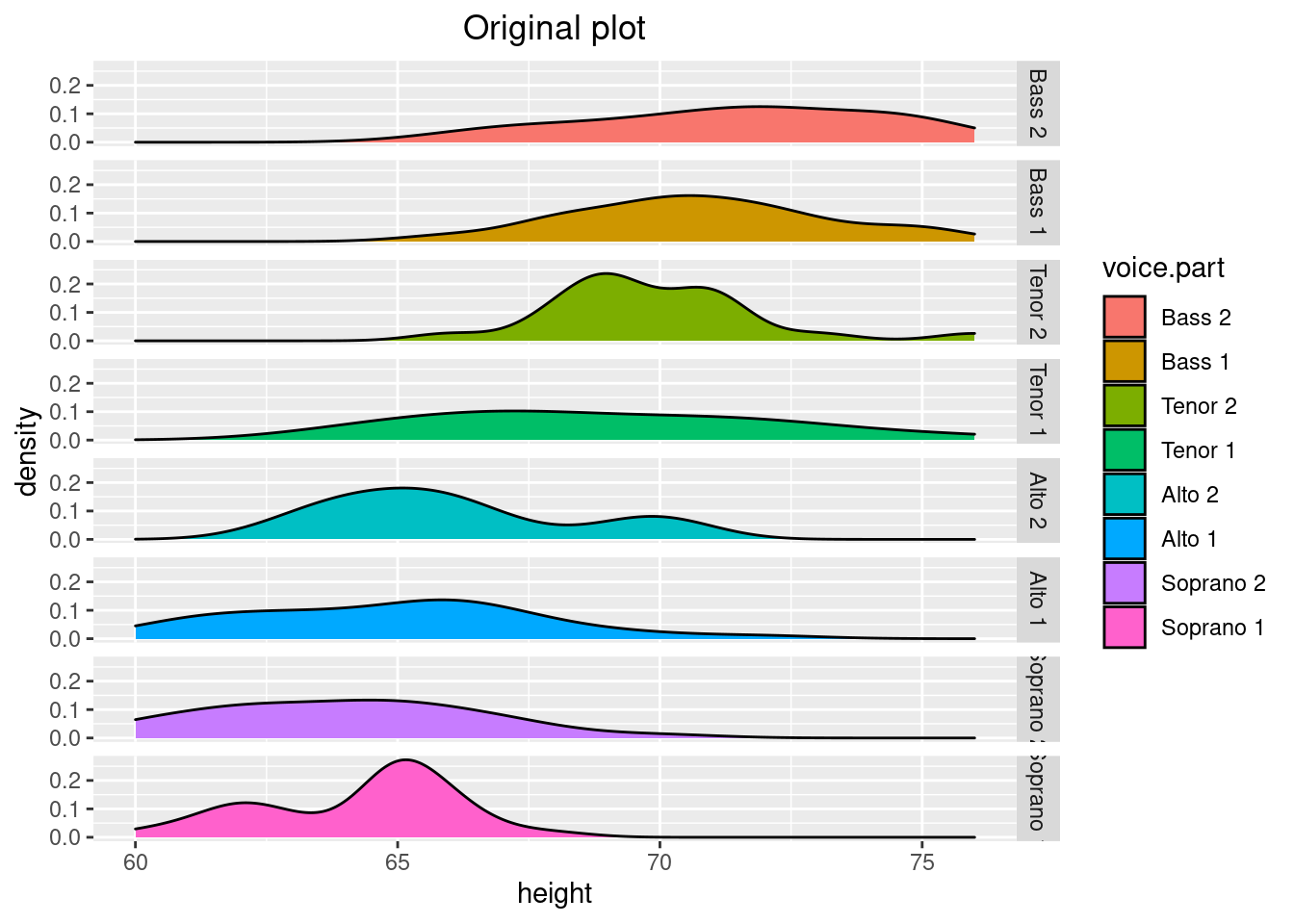
library(plotly)
p <- ggplot(data=lattice::singer,aes(x=height,fill=voice.part))+
  geom_density()+
  facet_grid(voice.part~.)+
  ggtitle('Original plot using ggplotly') +
  theme(plot.title = element_text(hjust = 0.5))
(gg <- ggplotly(p))
45.5 rCharts
rCharts may be the most famous or popular package for interactive diagrams. It is an R package to create, customize and publish interactive javascript visualizations from R using a familiar lattice style plotting interface(Cited from https://ramnathv.github.io/rCharts/). And the way to use its functions are quite straightforward - type is used to define the specific diagram type, formulation and data is used to specify which data to use and how to use.
45.5.2 hPlot
Highcharts is a pure Javascript library for charting, supporting most types of charts: line charts, graphs, region charts, region charts, bar charts, pie charts, scatter charts, etc. The hPlot function is provided in the rCharts package to achieve this. Below is an example where I plotted bubble plots of student height and pulse beats per minute, using the age as a variable to adjust bubble size.
library(rCharts)
a <- hPlot(Pulse ~ Height, data = MASS::survey, type = "bubble",title = "hPlot Example", subtitle = "bubble chart",size = "Age", group = "Exer")
a$colors('rgba(223, 83, 83, .5)', 'rgba(119, 152, 191, .5)','rgba(60, 179, 113, .5)')
a$chart(zoomType = "xy")
a$exporting(enabled = T)
#a$save("p1.2.html", standalone = TRUE)
a
45.5.3 nPlot
library(rCharts)
hair_eye_male <- subset(as.data.frame(HairEyeColor), Sex == "Male")
hair_eye_male[,1] <- paste0("Hair",hair_eye_male[,1])
hair_eye_male[,2] <- paste0("Eye",hair_eye_male[,2])
n1 <- nPlot(Freq ~ Hair, group = "Eye", data = hair_eye_male,type = "multiBarChart")
#n1$save("p1.3.html", standalone = TRUE)
n1
More detailed tutorials and examples can be found here.http://ramnathv.github.io/rCharts//https://github.com/ramnathv/rCharts/tree/master/demo
45.6 reCharts
reCharts means redefine. The reason behind the name is that this package gives users different experience in design. It not only redefine React design, but also redefines its composition and configuration.
As the developers mentioned when they introduced this package, the main problems during creating diagrams maybe as below:
(1) Too much parameter can be used, which not only make the process more complicated but also cause some misunderstandings.
(2) Styles between diagrams vary a lot and is hard to unify. For example, someone may ask - Why is the pillar of the bar chart a triangle?
reCharts sovles these problems use following methods: (1) Declarative tags make writing charts as easy as writing HTML
(2) Configuration items that are close to native SVG make configuration items more natural
(3) Interface API, to solve a variety of personalized needs
library(recharts)
names(iris) = gsub("\\.", "", names(iris))
p <- echart(data=iris,x = ~PetalLength, y = ~PetalWidth,series = ~Species,type = 'scatter')
p
hair_eye_male <- subset(as.data.frame(HairEyeColor), Sex == "Male")
hair_eye_male[,1] <- paste0("Hair",hair_eye_male[,1])
hair_eye_male[,2] <- paste0("Eye",hair_eye_male[,2])
p <- echart(data = hair_eye_male, x = ~Hair, y = ~Freq,  series = ~Eye,
       type = 'bar', palette='fivethirtyeight',
       xlab = 'Hair', ylab = 'Freq')
p
More detailed tutorials and examples can be found here.https://recharts.org/en-US/
45.7 highcharter
The final package in this document is highcharter. Highcharter is a chart library written in pure JavaScript that makes it easy to add interactive charts to Web sites or Web applications. In this section, more complicated diagram will be introduced and I will try to figure the procedures in a more detailed way.(cite fromhttps://zhuanlan.zhihu.com/p/42430990)
m <- c(1746181,1884428,2089758,2222362,2537431,2507081,2443179,2664537,3556505,3680231, 3143062 ,2721122, 2229181 ,2227768,
       2176300, 1329968 , 836804,354784,90569,28367,3878)
f <- c(1656154, 1787564, 1981671, 2108575, 2403438, 2366003, 2301402, 2519874,3360596, 3493473, 3050775, 2759560, 2304444,
       2426504, 2568938, 1785638,1447162, 1005011, 330870, 130632, 21208)
class <- c('0-4', '5-9', '10-14', '15-19','20-24', '25-29', '30-34', '35-39', '40-44','45-49', '50-54','55-59', '60-64',
           '65-69', '70-74', '75-79', '80-84', '85-89', '90-94','95-99', '100 + ')

highchart() %>%
    hc_xAxis(list(categories = class,
        reversed = FALSE, # whether to flip the coordinate
        labels = list(step = 1)),
      list(
        opposite = TRUE, # ajust the position of the coordinate
        categories = class,
        reversed = FALSE,
        linkedTo = 0,
        labels = list(step = 1))
    ) %>%
  hc_plotOptions(series = list(borderWidth = 0))%>%
  hc_yAxis(
    labels = list(formatter = JS("function () { return (Math.abs(this.value) / 1000000) + 'M';}")),
    min = -4000000,max = 4000000)%>%# give the range of the x-axis
  hc_tooltip(formatter = JS("function () {
                                   return '<b>' + this.series.name + ', age ' + this.point.category + '</b><br/>' +
                                     'popluation: ' + Highcharts.numberFormat(Math.abs(this.point.y), 0);}"))%>%
  hc_title(text = "Popluation in 2015 Germany",align="center")%>%
  hc_plotOptions(series= list(stacking = "normal")) %>%
  # set the value to be negative to make them display in a same coordinate
  hc_add_series(name = "Male",data = -m, type = "bar") %>%
  hc_add_series(name = "Female",data = f,type = "bar") %>%
  hc_add_theme(hc_theme_538())
text_data <- data.table(text =c("Brazil",    "Canada",  "Mexico",  "USA",   "Switerzeland",  "France",   "Spain",  "British",   "South Africa",   "Russia",  "Germany", "Iceland",   "Korean",  "China",   "India",   "Japan"),
                        weight =c(2,    3,  1,  1,  4,  5,  4,  3,  1,  1,  2,  3,  2,  6,  1,  1))

highchart() %>%
  hc_title(text = "World Cloud") %>%
  hc_add_series(data = text_data,type = "wordcloud",name= "Score",hcaes(name = text,weight = weight)) %>%
  hc_add_theme(hc_theme_flat())
explorer_rate <- data.table(name = c('Firefox','IE','Chrome','Safari','Opera','other'),
                            rate = c(45,    26.8,   12.8,   8.5,6.2,0.7))

highchart() %>%
  hc_title(
    #“<br>” can help change a line
    text = "Web broswer<br>Percentage",
    #position of title in horizontal axis
    align = "center",
    #position of title in vertical axis
    verticalAlign = "middle",
    y = 60) %>%
  hc_plotOptions(pie = list(
    dataLabels = list(
      #show the label
      enabled = TRUE,
      #change the position
      distance = -50,
      style = list(fontWeight = "bold",color = "white")),
    #the start angle of the chart
    startAngle = -90,
    #the end angle of the chart
    endAngle = 90,
    center = c('50%','75%')))%>%
  hc_tooltip(
    headerFormat = "{series.name}<br>",
    pointFormat = "{point.name}: <b>{point.percentage:.1f}%</b>")%>%
  hc_add_series(explorer_rate,type = "pie",hcaes(name = name, y = rate),name = "percentage",
                #control the size
                innerSize = "50%") %>%
  hc_add_theme(hc_theme_google())
type <- c("Sales", "Marketing", "Development", "Support","IT","Administration")
actual <- c(50000, 39000, 42000, 31000, 26000, 14000)
plan <- c(43000, 19000, 60000, 35000, 17000, 10000)

highchart() %>%
  #set as polar coordinates
  hc_chart(polar = TRUE,type = "line") %>%
  hc_title(text = "Budget and Expenditure",x=-60) %>%
  hc_pane(size = "80%") %>%
  hc_legend(align = "right",verticalAlign = "top",y = 70,layout = "vertical") %>%
  hc_xAxis(categories = type,
           #hide the horizontal line
           lineWidth = 0,
           #rotate to match the vertices of the polygon
           tickmarkPlacement = "on") %>%
  hc_yAxis(#set as polygon
           gridLineInterpolation = "polygon",
           #hide the vertial line
           lineWidth = 0,
           min = 0) %>%
  hc_tooltip(#show the result for two different type in the same line
             shared = TRUE,
             pointFormat = '<span style="color:{series.color}">{series.name}: <b>${point.y:,.0f}</b><br/>')%>%
  hc_add_series(name = "Expenditure",actual) %>%
  hc_add_series(name = "Budget",plan) %>%
  hc_add_theme(hc_theme_google())