64 Introduction to models and prediction evaluation
Yi Duan
In this introduction, we will introduce the profit model, logit model and tree models. Moreover, we will use a specific example to show how they are used in R. To compare these models, we will introduce ROC to evaluate their predictions in the example.
64.1 Models for binomial data
64.1.1 Profit model
In statistics, a probit model is a type of regression where the dependent variable can take only two values. The word is a portmanteau, coming from probability + unit. The purpose of the model is to estimate the probability that an observation with particular characteristics will fall into a specific one of the categories; moreover, classifying observations based on their predicted probabilities is a type of binary classification model.
A probit model is a popular specification for a binary response model. As such it treats the same set of problems as does logistic regression using similar techniques. When viewed in the generalized linear model framework, the probit model employs a probit link function. It is most often estimated using the maximum likelihood procedure, such an estimation being called a probit regression.
There is an underlying mechanism, there is a variable y, that is distributed normally (denoted \(\phi\)()). When y is greater than a threshold, we get an observation. The probability changes because the mean \(\mu\) is a linear function of the conditioning variables =x’\(\beta\).
64.1.2 Logit model
In statistics, the logistic model (or logit model) is used to model the probability of a certain class or event existing such as pass/fail, win/lose, alive/dead or healthy/sick. This can be extended to model several classes of events such as determining whether an image contains a cat, dog, lion, etc. Each object being detected in the image would be assigned a probability between 0 and 1, with a sum of one.
Logistic regression is a statistical model that in its basic form uses a logistic function to model a binary dependent variable, although many more complex extensions exist. In regression analysis, logistic regression is estimating the parameters of a logistic model (a form of binary regression). Mathematically, a binary logistic model has a dependent variable with two possible values, such as pass/fail which is represented by an indicator variable, where the two values are labeled “0” and “1”. In the logistic model, the log-odds (the logarithm of the odds) for the value labeled “1” is a linear combination of one or more independent variables (“predictors”); the independent variables can each be a binary variable (two classes, coded by an indicator variable) or a continuous variable (any real value). The defining characteristic of the logistic model is that increasing one of the independent variables multiplicatively scales the odds of the given outcome at a constant rate, with each independent variable having its own parameter; for a binary dependent variable this generalizes the odds ratio.
The log odds is a linear function of the conditioning variables, ln(p/(1-p)) =x’\(\beta\)
So p=exp(x’\(\beta\))/(1+exp(x’\(\beta\)))
64.1.3 How to fit these and choose models
- Likelihood
- The product of the densities (or probability mass function) evaluated at the data
-
\(L(x)=f(x_1)f(x_2)...f(x_n)=\prod_{i=1}^{n} f(x_i)\)
- We want to maximize this.
- The product of the densities (or probability mass function) evaluated at the data
- Log likelihood works better
-
\(l(x)=ln(f(x_1)f(x_2)...f(x_n))=\sum_{i=1}^{n} ln(f(x_i))\)
-
\(l(x)=ln(f(x_1)f(x_2)...f(x_n))=\sum_{i=1}^{n} ln(f(x_i))\)
- If f is contained in g
- 2*ln(L(x|f)/L(x|g))~\(\chi^2_{n(g)-n(f)}\), n(f)= number of parameters in f. This is like sums of squares, just need a base likelihood g. The package glm, provides this. And for nested models we can compare likelihood differences.
- Deviance(2(ln(x,f)-ln(x,x)) allows direct comparison between models.
64.1.4 We will use GLM to fit and analyze models
GLM is used to fit generalized linear models, specified by giving a symbolic description of the linear predictor and a description of the error distribution. Family objects provide a convenient way to specify the details of the models used by functions such as glm. Link is a specification for the model link function.
Let’s take a look at the Default data first.
Default[1:3,]## default student balance income
## 1 No No 729.5265 44361.63
## 2 No Yes 817.1804 12106.13
## 3 No No 1073.5492 31767.14Student or non-student status may have a very significant effect, so we can model the effects on default of balance and income.
1. For all the data
2. Separately for the student and the non-student data
Logit Model
To use the logit model, we need to set family to binomial and link to logit.
Default.logit.out<-glm(default~balance+income,family=binomial(link=logit),Default)
summary(Default.logit.out)
##
## Call:
## glm(formula = default ~ balance + income, family = binomial(link = logit),
## data = Default)
##
## Deviance Residuals:
## Min 1Q Median 3Q Max
## -2.4725 -0.1444 -0.0574 -0.0211 3.7245
##
## Coefficients:
## Estimate Std. Error z value Pr(>|z|)
## (Intercept) -1.154e+01 4.348e-01 -26.545 < 2e-16 ***
## balance 5.647e-03 2.274e-04 24.836 < 2e-16 ***
## income 2.081e-05 4.985e-06 4.174 2.99e-05 ***
## ---
## Signif. codes: 0 '***' 0.001 '**' 0.01 '*' 0.05 '.' 0.1 ' ' 1
##
## (Dispersion parameter for binomial family taken to be 1)
##
## Null deviance: 2920.6 on 9999 degrees of freedom
## Residual deviance: 1579.0 on 9997 degrees of freedom
## AIC: 1585
##
## Number of Fisher Scoring iterations: 8Logit, just students
Student.Default<-filter(Default,student=="Yes")
Default.logit.out.stu<-glm(default~balance+income,family=binomial(link=logit),Student.Default)
summary(Default.logit.out.stu)
##
## Call:
## glm(formula = default ~ balance + income, family = binomial(link = logit),
## data = Student.Default)
##
## Deviance Residuals:
## Min 1Q Median 3Q Max
## -2.1244 -0.1674 -0.0691 -0.0265 3.3252
##
## Coefficients:
## Estimate Std. Error z value Pr(>|z|)
## (Intercept) -1.151e+01 8.107e-01 -14.194 <2e-16 ***
## balance 5.598e-03 3.774e-04 14.832 <2e-16 ***
## income 1.585e-05 2.610e-05 0.607 0.544
## ---
## Signif. codes: 0 '***' 0.001 '**' 0.01 '*' 0.05 '.' 0.1 ' ' 1
##
## (Dispersion parameter for binomial family taken to be 1)
##
## Null deviance: 1046.85 on 2943 degrees of freedom
## Residual deviance: 563.03 on 2941 degrees of freedom
## AIC: 569.03
##
## Number of Fisher Scoring iterations: 8Logit, no students
NonStudent.Default<-filter(Default,student=="No")
Default.logit.out.nstu<-glm(default~balance+income,family=binomial(link=logit),NonStudent.Default)
summary(Default.logit.out.nstu)
##
## Call:
## glm(formula = default ~ balance + income, family = binomial(link = logit),
## data = NonStudent.Default)
##
## Deviance Residuals:
## Min 1Q Median 3Q Max
## -2.4897 -0.1316 -0.0502 -0.0181 3.7600
##
## Coefficients:
## Estimate Std. Error z value Pr(>|z|)
## (Intercept) -1.094e+01 5.752e-01 -19.015 <2e-16 ***
## balance 5.818e-03 2.938e-04 19.803 <2e-16 ***
## income 1.597e-06 8.670e-06 0.184 0.854
## ---
## Signif. codes: 0 '***' 0.001 '**' 0.01 '*' 0.05 '.' 0.1 ' ' 1
##
## (Dispersion parameter for binomial family taken to be 1)
##
## Null deviance: 1861.8 on 7055 degrees of freedom
## Residual deviance: 1008.0 on 7053 degrees of freedom
## AIC: 1014
##
## Number of Fisher Scoring iterations: 8Modeling student
Default.logit.out.allvar<-glm(default~balance+income+student,family=binomial(link=logit),Default)
summary(Default.logit.out.allvar)
##
## Call:
## glm(formula = default ~ balance + income + student, family = binomial(link = logit),
## data = Default)
##
## Deviance Residuals:
## Min 1Q Median 3Q Max
## -2.4691 -0.1418 -0.0557 -0.0203 3.7383
##
## Coefficients:
## Estimate Std. Error z value Pr(>|z|)
## (Intercept) -1.087e+01 4.923e-01 -22.080 < 2e-16 ***
## balance 5.737e-03 2.319e-04 24.738 < 2e-16 ***
## income 3.033e-06 8.203e-06 0.370 0.71152
## studentYes -6.468e-01 2.363e-01 -2.738 0.00619 **
## ---
## Signif. codes: 0 '***' 0.001 '**' 0.01 '*' 0.05 '.' 0.1 ' ' 1
##
## (Dispersion parameter for binomial family taken to be 1)
##
## Null deviance: 2920.6 on 9999 degrees of freedom
## Residual deviance: 1571.5 on 9996 degrees of freedom
## AIC: 1579.5
##
## Number of Fisher Scoring iterations: 8Neither students nor non students have a dependence on income. Balance has nearly the same coefficient in all the models so with student in the model, so we may drop the income.
Modeling without income
Default.logit.out.noincome<-glm(default~balance+student,family=binomial(link=logit),Default)
summary(Default.logit.out.noincome)
##
## Call:
## glm(formula = default ~ balance + student, family = binomial(link = logit),
## data = Default)
##
## Deviance Residuals:
## Min 1Q Median 3Q Max
## -2.4578 -0.1422 -0.0559 -0.0203 3.7435
##
## Coefficients:
## Estimate Std. Error z value Pr(>|z|)
## (Intercept) -1.075e+01 3.692e-01 -29.116 < 2e-16 ***
## balance 5.738e-03 2.318e-04 24.750 < 2e-16 ***
## studentYes -7.149e-01 1.475e-01 -4.846 1.26e-06 ***
## ---
## Signif. codes: 0 '***' 0.001 '**' 0.01 '*' 0.05 '.' 0.1 ' ' 1
##
## (Dispersion parameter for binomial family taken to be 1)
##
## Null deviance: 2920.6 on 9999 degrees of freedom
## Residual deviance: 1571.7 on 9997 degrees of freedom
## AIC: 1577.7
##
## Number of Fisher Scoring iterations: 8Using the logit model the probability of default seems to be only a function of student status and balance, not income.
Probit Model
To use the probit model, we need to set family to binomial and link to probit.
Default.logit.out.allvar<-glm(default~balance+income+student,family=binomial(link=probit),Default)
summary(Default.logit.out.allvar)
##
## Call:
## glm(formula = default ~ balance + income + student, family = binomial(link = probit),
## data = Default)
##
## Deviance Residuals:
## Min 1Q Median 3Q Max
## -2.2226 -0.1354 -0.0321 -0.0044 4.1254
##
## Coefficients:
## Estimate Std. Error z value Pr(>|z|)
## (Intercept) -5.475e+00 2.385e-01 -22.960 <2e-16 ***
## balance 2.821e-03 1.139e-04 24.774 <2e-16 ***
## income 2.101e-06 4.121e-06 0.510 0.6101
## studentYes -2.960e-01 1.188e-01 -2.491 0.0127 *
## ---
## Signif. codes: 0 '***' 0.001 '**' 0.01 '*' 0.05 '.' 0.1 ' ' 1
##
## (Dispersion parameter for binomial family taken to be 1)
##
## Null deviance: 2920.6 on 9999 degrees of freedom
## Residual deviance: 1583.2 on 9996 degrees of freedom
## AIC: 1591.2
##
## Number of Fisher Scoring iterations: 8Probit no income
Default.probit.out.noincome<-glm(default~balance+student,family=binomial(link=probit),Default)
summary(Default.probit.out.noincome)
##
## Call:
## glm(formula = default ~ balance + student, family = binomial(link = probit),
## data = Default)
##
## Deviance Residuals:
## Min 1Q Median 3Q Max
## -2.2056 -0.1353 -0.0322 -0.0044 4.1374
##
## Coefficients:
## Estimate Std. Error z value Pr(>|z|)
## (Intercept) -5.3918818 0.1728730 -31.190 < 2e-16 ***
## balance 0.0028215 0.0001138 24.784 < 2e-16 ***
## studentYes -0.3429201 0.0743964 -4.609 4.04e-06 ***
## ---
## Signif. codes: 0 '***' 0.001 '**' 0.01 '*' 0.05 '.' 0.1 ' ' 1
##
## (Dispersion parameter for binomial family taken to be 1)
##
## Null deviance: 2920.6 on 9999 degrees of freedom
## Residual deviance: 1583.5 on 9997 degrees of freedom
## AIC: 1589.5
##
## Number of Fisher Scoring iterations: 8Logit has mildly sharper dependence on both balance and student status for fit than Probit.
Income doesn’t matter, but student status does.
What else matters is the balance owed.
Increased balance: default more likely.
Student status: default less likely.
64.2 Receiver Operating Characteristic
Definitions:
condition positive (P): the number of real positive cases in the data
condition negative (N): the number of real negative cases in the data
true positive (TP): eqv. with hit
true negative (TN): eqv. with correct rejection
false positive (FP): eqv. with false alarm, type I error or underestimation
false negative (FN): eqv. with miss, type II error or overestimation
ROC plots true positive rate vs false positive rate as a function of threshold.
true positive rate TPR=TP/(TP+FN)
false positive rate FPR=FP/(FP+TN)
64.2.1 ROC in R
The function of ROC can build a ROC curve and return a “roc” object, a list of class “roc”, which can be printed and plotted. In the function of ROC, the first parameter is response, and the second parameter is predictor.
#Create a test and train data set
v1<-sort(sample(10000,6000))
Default.train<-Default[v1,]
Default.test<-Default[-v1,]
#Create a logit model using glm
Default.train.out.noincome<-glm(default~balance+student,family=binomial(link=logit),Default.train)
#Predict the test data set
Default.pred<-predict(Default.train.out.noincome,Default.test,type="response")
roc(Default.test$default,Default.pred,plot=T)
##
## Call:
## roc.default(response = Default.test$default, predictor = Default.pred, plot = T)
##
## Data: Default.pred in 3866 controls (Default.test$default No) < 134 cases (Default.test$default Yes).
## Area under the curve: 0.9471
Default.pred.self<-predict(Default.train.out.noincome,type="response")
roc.train.str<-roc(Default.train$default,Default.pred.self)
lines.roc(roc.train.str,type="lines",col=2)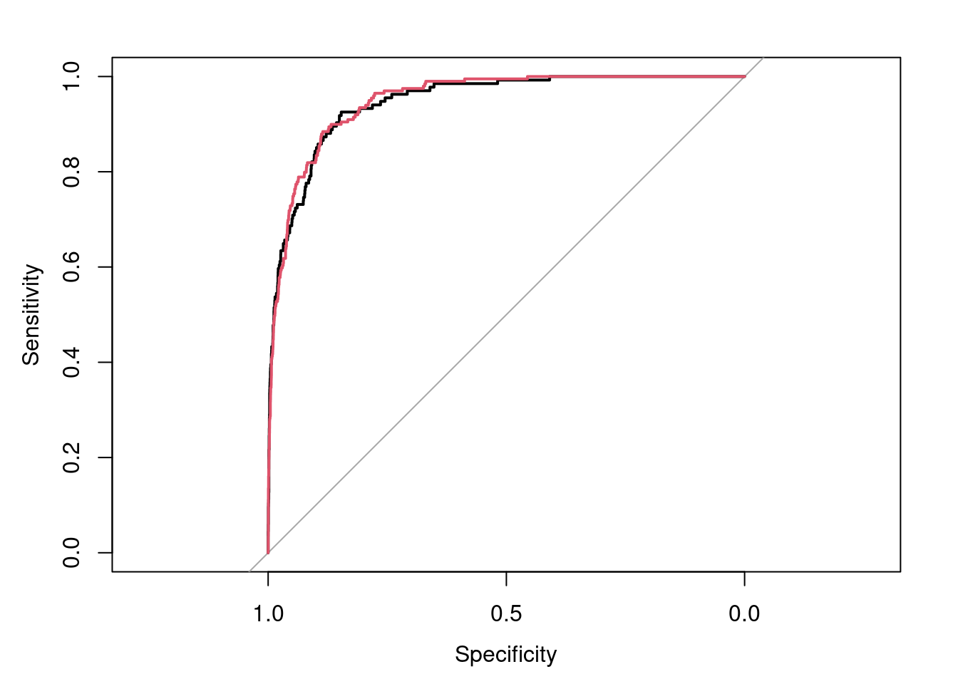
In the plot, Sensitivity=True Positive Rate, Specificity=False Positive Rate.
64.3 Classification and Regression Trees
64.3.1 Recursive Partitioning
Recursive partitioning can be used either with regression or binary data.
We will introduce three of the choices.
* tree - a few more options
* rpart - nicer graphics
* randomForest - different approach
Let’s see how these models work on the Auto data.
64.3.2 Basic Trees
There are p dimensions, n data points.
Step 1: cycle through all p dimensions, all n-1 possible splits on those dimensions, Choose the 1 that now gives the most improvement in:
* Sum of squares for regression
* Likelihood for other models
Step 2: for each data set created, redo step 1 but select the 1 best division.
Go until some criteria is met.
Problems: Easy to overfit
Step 1, prune back using cross validation to evaluate error. (chop off parts of tree somewhat automatic)
#Create a training sample for Auto
I1<-sample(392,200)
Auto1<-Auto[I1,]
Auto2<-Auto[-I1,]
dum0tree<-tree(mpg~cylinders+displacement+horsepower+weight+year+acceleration,data=Auto1)
plot(dum0tree)
text(dum0tree)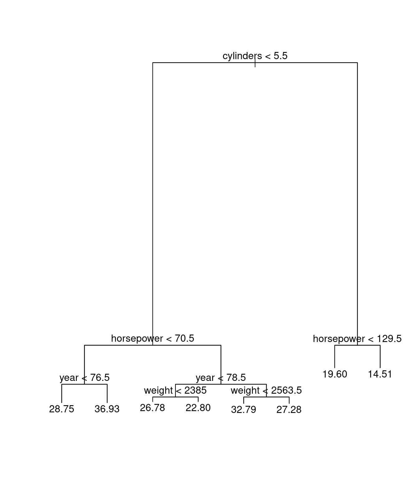
64.3.3 Rpart: Recursive Partitioning and Regression Trees
dum0rpart<-rpart(mpg~cylinders+displacement+horsepower+weight+year+acceleration,data=Auto1)
plot(dum0rpart)
text(dum0rpart)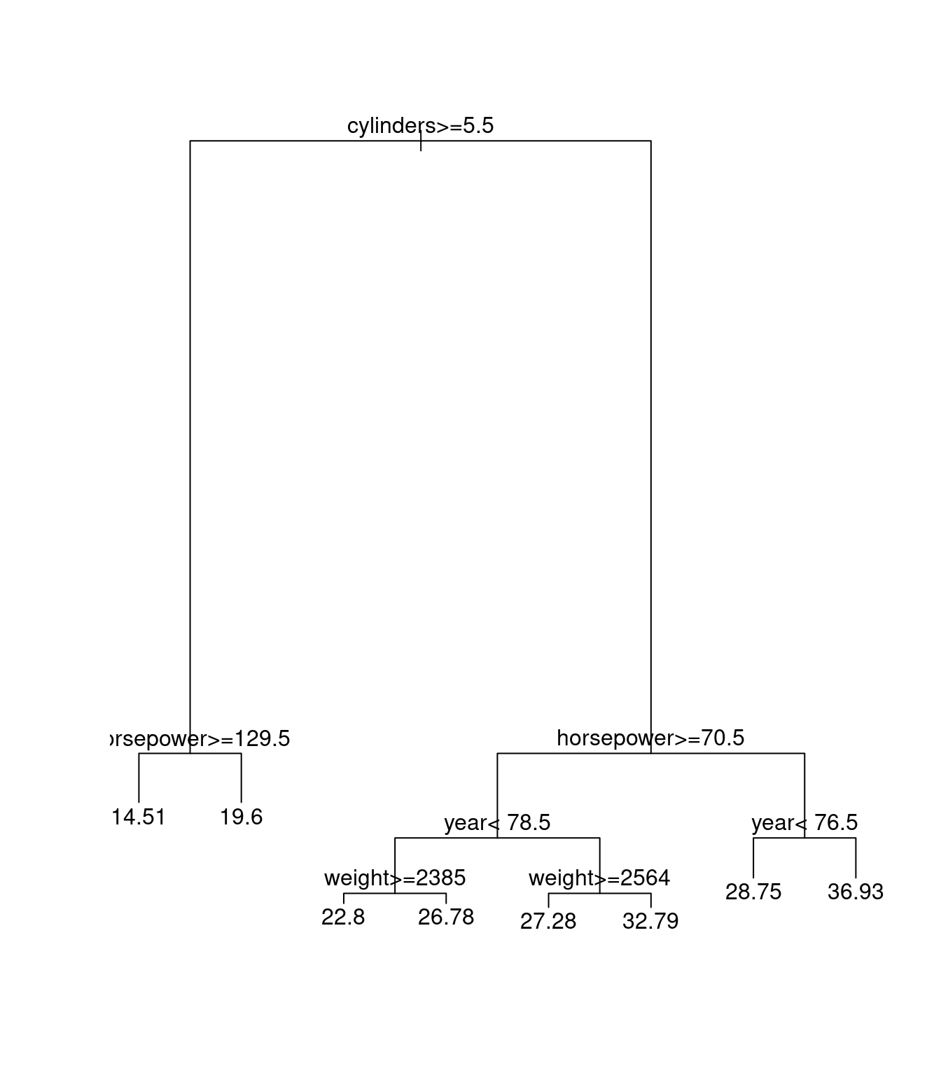
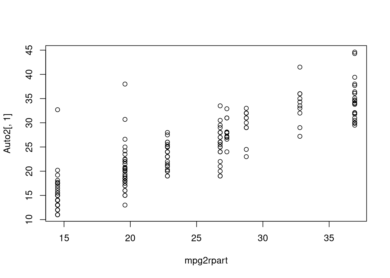
Here we can see that tree and rpart are doing the same thing in regression.
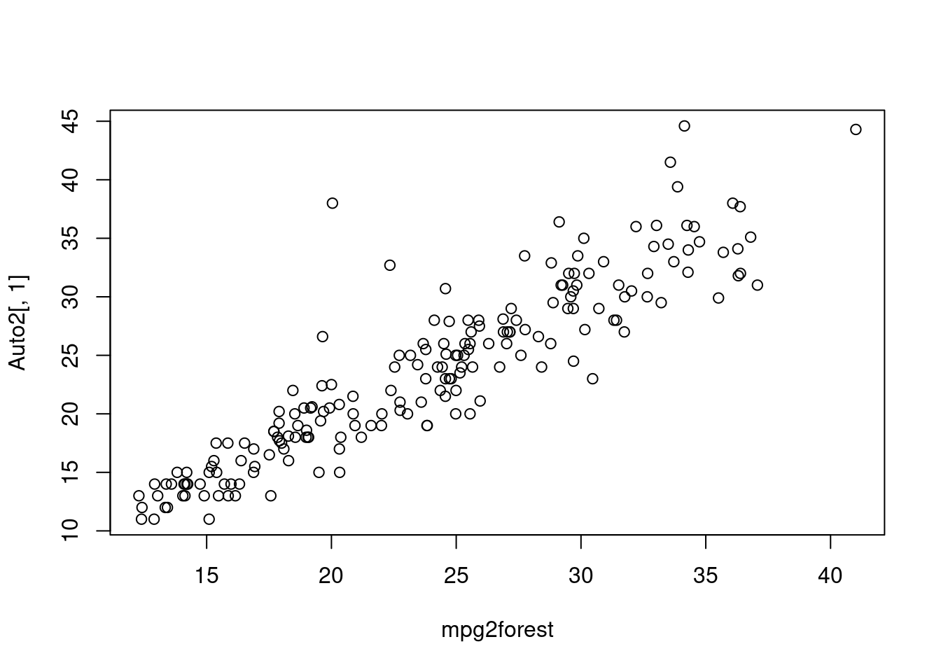
64.3.4 Random Forests
There are p dimensions, n data points.
Step 1: cycle through all a random selection of the dimensions, and a random selection of n-1 possible splits on those dimensions, Choose the 1 that now gives the most improvement in :
* Sum of squares for regression
* Likelihood for other models
Step 2: for each data set created, redo step 1 but with new randomly selected dimensions and divisions.
Step 3: repeat 1 and 2 on original data until a number of random trees are made.
For classification, each tree gets 1 vote (or is averaged) for the prediction of the new data.
NICE result, large n big forest, does not over fit.
dum0forest<-randomForest(mpg~cylinders+displacement+horsepower+weight+year+acceleration,data=Auto1)
plot(dum0forest)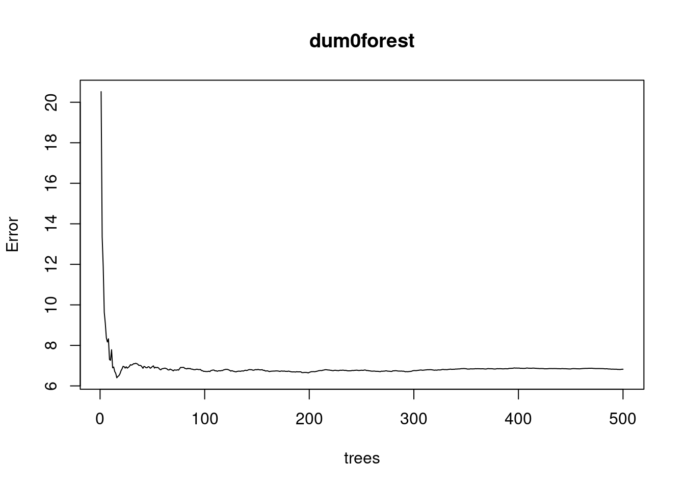
Plot here tells us if forest is large enough for the error to converge.
64.3.5 We can use tree, rpart, and random forest on binary data too
Let’s go back to the Default data and create the model of train data set using different methods.
Basic Trees
Default.tree.train.out.noincome<-tree(default~balance+student,Default.train)
plot(Default.tree.train.out.noincome)
text(Default.tree.train.out.noincome)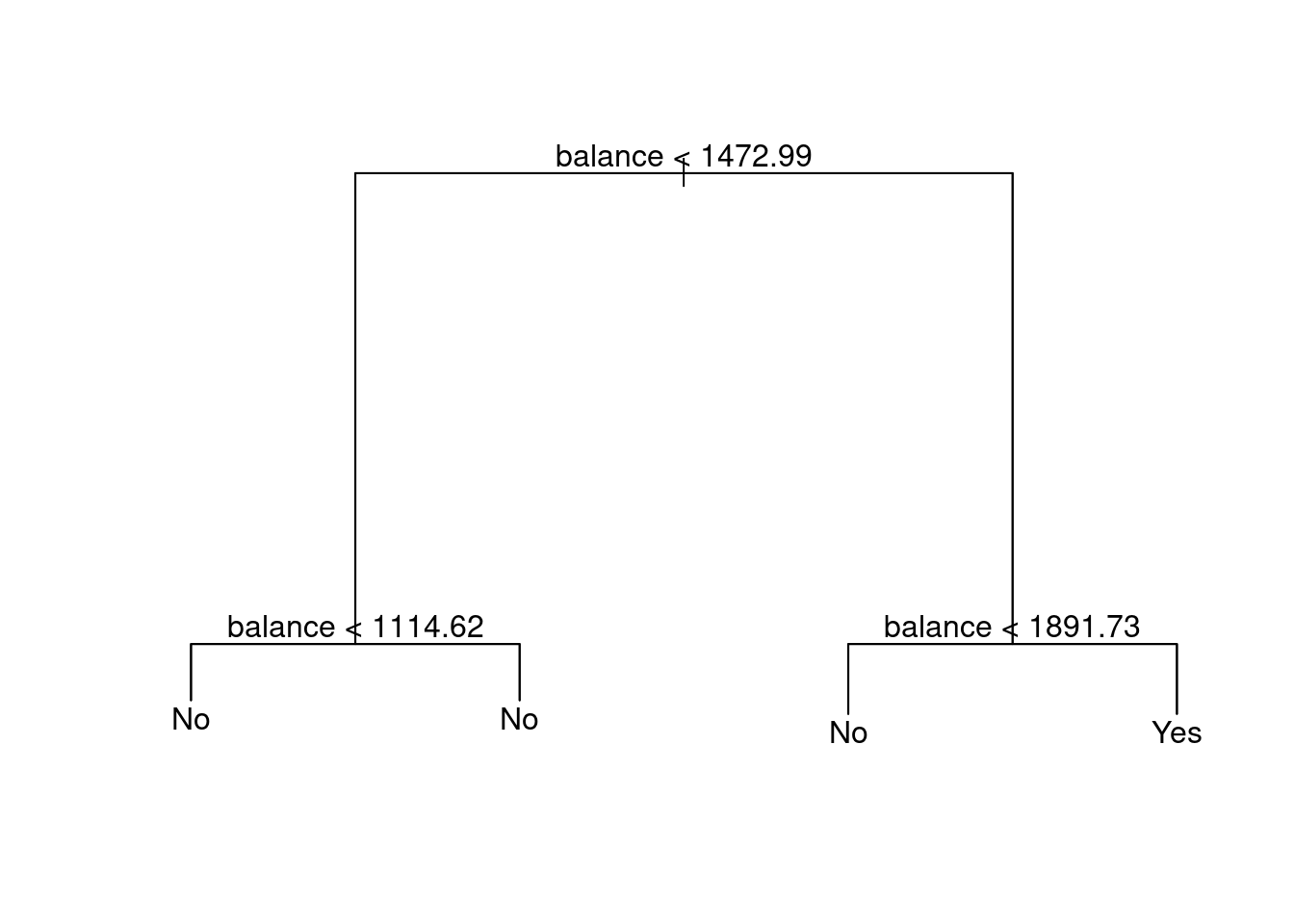
Rpart
Default.rpart.train.out.noincome<-rpart(default~balance+student,Default.train)
plot(Default.rpart.train.out.noincome)
text(Default.rpart.train.out.noincome)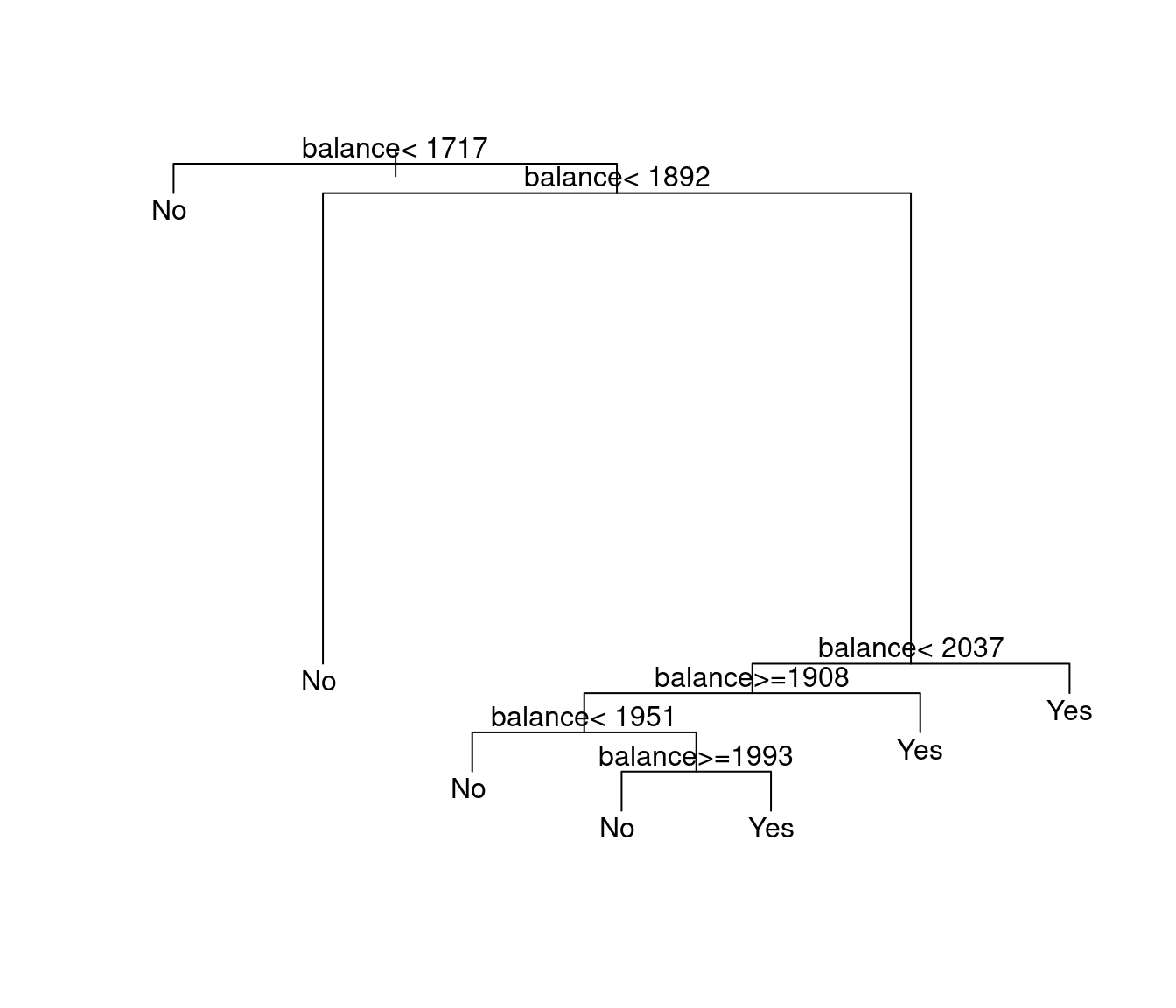
Random Forests
Default.rf.train.out.noincome<-randomForest(default~balance+student,Default.train)
plot(Default.rf.train.out.noincome)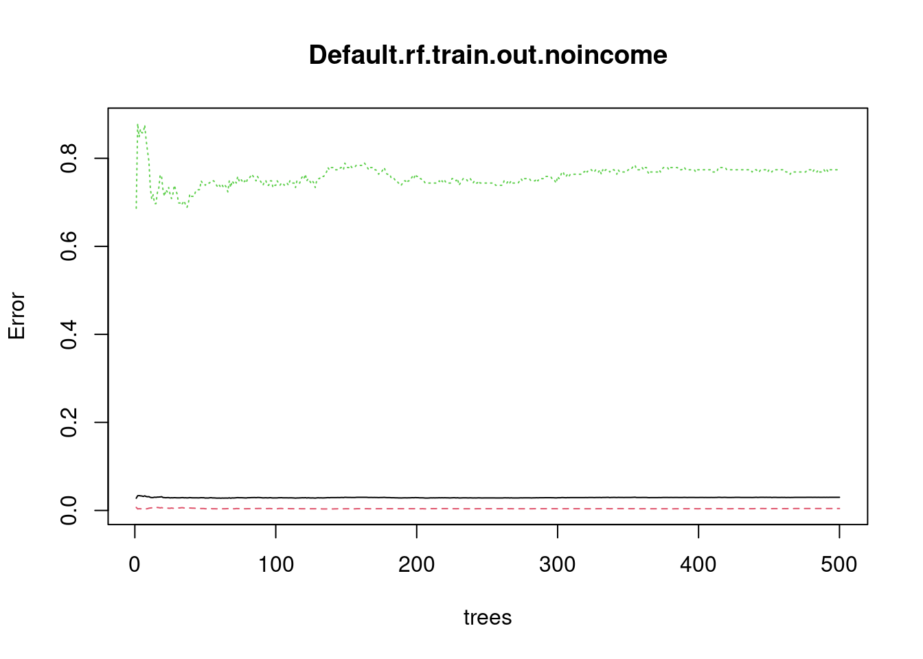
64.3.6 ROC on tree, rpart, and random forest
#Predict the test data set
tree.test.pred<-predict(Default.tree.train.out.noincome,Default.test)
rpart.test.pred<-predict(Default.rpart.train.out.noincome,Default.test)
Default.rf.test.pred<-predict(Default.rf.train.out.noincome,Default.test,type="prob")
#roc for tree
roc(Default.test$default,tree.test.pred[,2],plot=T)
##
## Call:
## roc.default(response = Default.test$default, predictor = tree.test.pred[, 2], plot = T)
##
## Data: tree.test.pred[, 2] in 3866 controls (Default.test$default No) < 134 cases (Default.test$default Yes).
## Area under the curve: 0.9224
#roc for rpart
roc.rpart.default.pred<-roc(Default.test$default,rpart.test.pred[,2])
lines.roc(roc.rpart.default.pred,type="lines",col=2)
print(roc.rpart.default.pred)
##
## Call:
## roc.default(response = Default.test$default, predictor = rpart.test.pred[, 2])
##
## Data: rpart.test.pred[, 2] in 3866 controls (Default.test$default No) < 134 cases (Default.test$default Yes).
## Area under the curve: 0.7755
#roc for random forest
rf.roc.pred<-roc(Default.test$default,Default.rf.test.pred[,2])
lines.roc(rf.roc.pred,type="lines",col=3)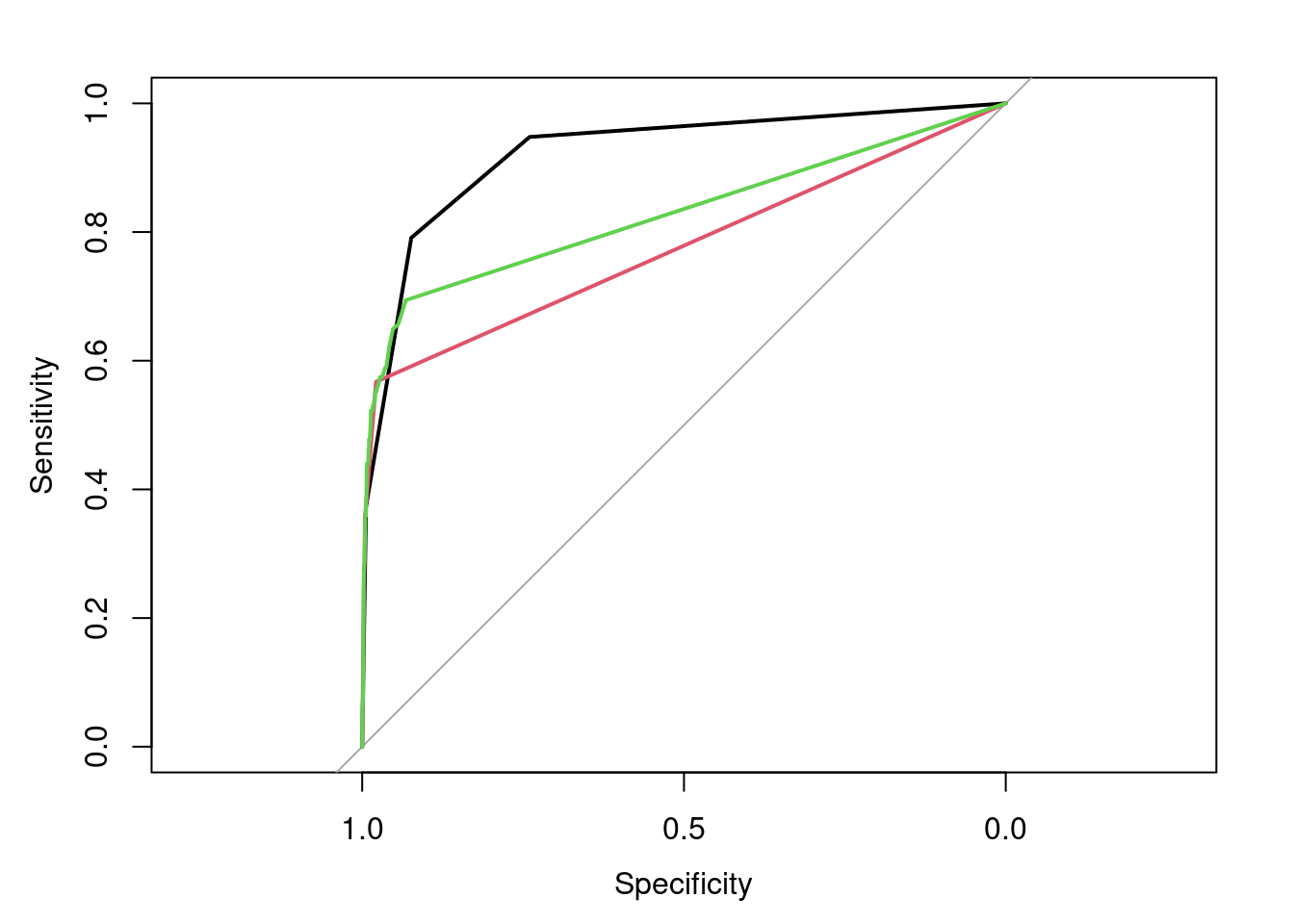
print(rf.roc.pred)##
## Call:
## roc.default(response = Default.test$default, predictor = Default.rf.test.pred[, 2])
##
## Data: Default.rf.test.pred[, 2] in 3866 controls (Default.test$default No) < 134 cases (Default.test$default Yes).
## Area under the curve: 0.8276We can compare the models and evaluate the predictions both from the ROC Area Under the Curve and the plot.
ROC AUC for the tree model is 0.9297, ROC AUC for the rpart model is 0.7479, and ROC AUC for the random forest model is 0.8172. 0.9297 > 0.8172 > 0.7479, so the tree model performs the best, while the rpart model performs the worst.
In this plot, the black line represents the tree model, the red line represents the rpart model, and the green line represents the random forest model. We can observe that the tree model has the best performance, while the rpart model has the worst performance.
These two results are consistent.
64.4 Reference
https://en.wikipedia.org/wiki/Probit_model
https://en.wikipedia.org/wiki/Logistic_regression#Definition_of_the_logistic_function
https://www.rdocumentation.org/packages/stats/versions/3.6.2/topics/glm
https://www.rdocumentation.org/packages/stats/versions/3.6.2/topics/family
https://en.wikipedia.org/wiki/Receiver_operating_characteristic
https://www.rdocumentation.org/packages/pROC/versions/1.16.2/topics/roc