71 Tutorial on R torch package
Wenbo Zhao
71.1 Introduction
Nowadays, deep learning technique has shown its ability in dealing with data intensive tasks such as image recognition, neural language processing and so on. In python, there are two famous deep learning frameworks: tensorflow[1] and pytorch[2]. While tensorflow provides R accessibility since 2017, torch is not available until the end of 2019[3]. Because of the use-friendliness of pytorch and the strong visualization ability of R, it is cool to combine them together. Here I would like to talk about how to use torch in R.
The torch ecosystem includes several packages. Torch package is the basic one that includes the basic data structure tensor, an N-d array of numbers, nn_modules that includes trainable weights and nnf_modules that are static ones. Luz package provides compact implementation of training procedure so that we do not need to write loops. Torchvision is a package especially designed for vision tasks that can crop or transform the images into suitable size to feed into the network.
71.2 Background
71.2.1 Deep Learning
Like linear regression, support vector machine and k-nearest neighbour, deep learning is also a kind of machine learning methods that can help us approximate the output or classify. All of these methods need a training dataset so that they can finetune their parameters and give the result of a new sample. One of the most important benefit of deep learning is the complexity of models that can abstract inner feature of samples and give precise prediction. It is said that with enough parameters, deep learning models can emulate any function between input and output. Of course this will cause overfitting problem and thus the size of model is set to be compatible with the size of input sample.
However, to present such a large deep learning model and its training process is not an easy task with traditional matrix multiplication. In such context, tensorflow and pytorch appears as an higher level API. With them, we can easily abstract a deep learning block and stacking these blocks together gives the complete network.
71.2.2 Convolution Neural Network
As is mentioned in the previous paragraph, a deep learning network is consisted of multiple blocks. For image classification task the most frequently used block is convolution neural network (CNN). Suppose we have a input of size \((N, C_{\mbox{in}}, H, W)\) and weight \(W\) of size \((C_{\mbox{out}}, C_{\mbox{in}}, k, k)\) with stride \(s\) and padding \(p\), the output size will be \((N, C_{\mbox{out}}, H_{\mbox{out}}, W_{\mbox{out}})\) where \[ H_{\mbox{out}} = \left\lfloor\frac{H + 2p - k}{s}\right\rfloor + 1 \\ W_{\mbox{out}} = \left\lfloor\frac{W + 2p - k}{s}\right\rfloor + 1 \] and \[ \mbox{out}[n, j, x, y] = \mbox{bias}_j + \mbox{inner_product}(W[j,:,:,:], \mbox{in}[n, :, 1+(x-1)s:1+(x-1)s+k, 1+(y-1)s:1+(y-1)s+k]) \] \(i.e.\) each output value is the inner product result of two 4-d array of size \([1,C_\mbox{in}, k, k]\) plus bias. This block is widely used in image tasks has achieved good result and is the basic unit in foundation networks Alexnet[4] and Resnet[5].
71.3 Implementation
71.3.1 Installation
To install torch in Rstudio, we should first install torch package. In our example, we also need luz and torchvision, therefore we run
install.packages("torch")
install.packages("torchvision")
install.packages("luz")
and then run
71.3.2 Fetching Dataset
In this example, we would like to identify the digits in the famous hand-written digit dataset MNIST using pure convolution neural network.
dir <- "./dataset/mnist"

train_ds <- mnist_dataset(
  dir,
  download = TRUE,
  transform = transform_to_tensor
)

test_ds <- mnist_dataset(
  dir,
  train = FALSE,
  transform = transform_to_tensor
)

train_dl <- dataloader(train_ds, batch_size = 128, shuffle = TRUE)
test_dl <- dataloader(test_ds, batch_size = 128)
The batch_size parameter is the number of inputs that are processed in parallel and its value is decided by the computation capacity of the processor. An example of the input is shown as follow:
image <- train_ds$data[1,1:28,1:28]
image_df <- melt(image)
ggplot(image_df, aes(x=Var2, y=Var1, fill=value))+
  geom_tile(show.legend = FALSE) +
  xlab("") + ylab("") +
  scale_fill_gradient(low="white", high="black")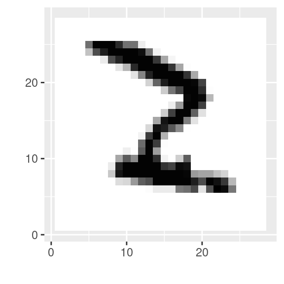
71.3.3 Building up the network
net <- nn_module(
  "Net",

  initialize = function() {
    self$conv1 <- nn_conv2d(1, 32, 3, 1)
    self$conv2 <- nn_conv2d(32, 64, 3, 1)
    self$dropout1 <- nn_dropout2d(0.25)
    self$dropout2 <- nn_dropout2d(0.5)
    self$fc1 <- nn_linear(9216, 128)
    self$fc2 <- nn_linear(128, 10)
  },

  forward = function(x) {
    x %>%                                  # N * 1 * 28 * 28
      self$conv1() %>%                     # N * 32 * 26 * 26
      nnf_relu() %>%
      self$conv2() %>%                     # N * 64 * 24 * 24
      nnf_relu() %>%
      nnf_max_pool2d(2) %>%                # N * 64 * 12 * 12
      self$dropout1() %>%
      torch_flatten(start_dim = 2) %>%     # N * 9216
      self$fc1() %>%                       # N * 128
      nnf_relu() %>%
      self$dropout2() %>%
      self$fc2()                           # N * 10
  }
)
The nn_module function requires 3 variables. A name variable which is an optional name for the module, an initialization function that includes all the accessaries that are needed in the network. In the example, they are all the convolution layers. The parameter of nn_conv2d are input channel \(C_\mbox{in}\), output channel \(C_\mbox{out}\), kernel size \(k\) and stride \(s\), which are described in previous sections. The padding \(p\) is set to 0 by default.
As is shown in the comment of the code, disregarding the batch size \(N\), the input size is an 28*28 image with only 1 input channel. After conv1, using the euqation of calculating \(H_\mbox{out}\) and \(W_\mbox{out}\), we can see that the size is 26*26 with 32 channels. After conv2, the shape is 24*24 with 64 channels. The max_pool2d(2) function selection the largest one from each 2*2 region to prevent overfit. After that the shape is 12*12 with 64 channels. The flatten function aligns them into a 9216 series and two linear layers finally get 10 values as the network output and the index of the largest one among them decides the output prediction digit.
71.3.4 Training
fitted <- net %>%
  setup(
    loss = nn_cross_entropy_loss(),
    optimizer = optim_adam,
    metrics = list(
      luz_metric_accuracy()
    )
  ) %>%
  fit(train_dl, epochs = 10, valid_data = test_dl)
Epoch 1/10
Train metrics: Loss: 0.2813 - Acc: 0.9146
Valid metrics: Loss: 0.0565 - Acc: 0.982
Epoch 2/10
Train metrics: Loss: 0.1055 - Acc: 0.9687
Valid metrics: Loss: 0.0424 - Acc: 0.985
Epoch 3/10
Train metrics: Loss: 0.0782 - Acc: 0.9756
Valid metrics: Loss: 0.0359 - Acc: 0.9872
Epoch 4/10
Train metrics: Loss: 0.0626 - Acc: 0.9815
Valid metrics: Loss: 0.0364 - Acc: 0.989
Epoch 5/10
Train metrics: Loss: 0.0563 - Acc: 0.983
Valid metrics: Loss: 0.0362 - Acc: 0.9889
Epoch 6/10
Train metrics: Loss: 0.0522 - Acc: 0.9831
Valid metrics: Loss: 0.0345 - Acc: 0.9892
Epoch 7/10
Train metrics: Loss: 0.0448 - Acc: 0.9861
Valid metrics: Loss: 0.029 - Acc: 0.9901
Epoch 8/10
Train metrics: Loss: 0.0415 - Acc: 0.9863
Valid metrics: Loss: 0.0307 - Acc: 0.9905
Epoch 9/10
Train metrics: Loss: 0.0361 - Acc: 0.9883
Valid metrics: Loss: 0.0289 - Acc: 0.9905
Epoch 10/10
Train metrics: Loss: 0.0337 - Acc: 0.9892
Valid metrics: Loss: 0.0286 - Acc: 0.990471.3.6 Saving the model
luz_save(fitted, "mnist-cnn.pt")71.4 Conclusion
Traning the model on R can gives us much merit since R can visualize the data easier and prettier than python. For example, we can plot the accuracy curve during the traning to see whether the model has converged, plot the distribution of trained weights to see the distribution difference in each layer, etc. Although some of the visualization method is already implemented with tensorboardX in python, I think it is still a beneficial attempt to train deep learning models on R.
71.5 Citation
[1] https://www.tensorflow.org/
[2] https://pytorch.org/
[3] https://torch.mlverse.org/
[4] Krizhevsky, Alex, Ilya Sutskever, and Geoffrey E. Hinton. “Imagenet classification with deep convolutional neural networks.” Advances in neural information processing systems 25 (2012): 1097-1105.
[5] He, Kaiming, et al. “Deep residual learning for image recognition.” Proceedings of the IEEE conference on computer vision and pattern recognition. 2016.