115 Tutorial for scatter plot with marginal distribution
Ziyu Fang
This tutorial introduces how to draw and customize scatter plots with marginal distribution map on the boundaries, including marginal histogram and marginal density plot.
There are mainly two approaches that are commonly used.
- The simple method: using two R libraries,
ggExtraandggplot2. In this way, we can generate marginal distribution map easily. - The advanced method: using two R libraries.
cowplotandggpubr. This approach allows users to have more flexiblity in designing and drawing plots.
115.1 Using ggExtra with ggplot2
115.1.1 Traditional Scatter Plot
Here is some sample code that draws simple 2D scatter plot. We assign a color to each species in the following plot.
p <- ggplot(iris) +
  geom_point(aes(x = Sepal.Length, y = Sepal.Width, color = Species), alpha = 0.6, shape = 16) +
  scale_color_brewer(palette = "Dark2") +
  theme_bw() +
  theme(legend.position = "bottom") +
  labs(x = "Sepal Length", y = "Sepal Width")
p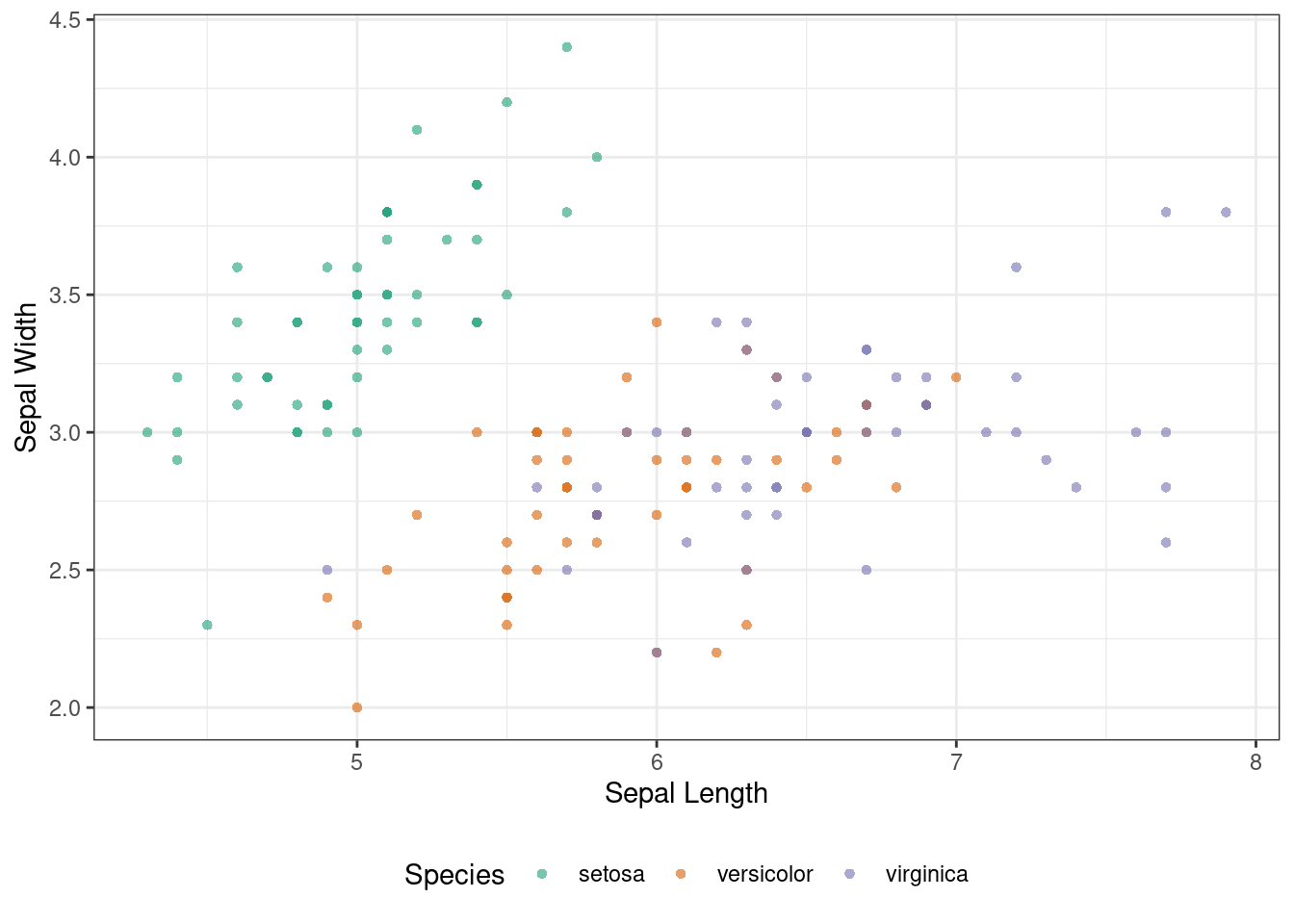
Using ggExtra and ggplot2 literally take one line of code to generate marginal histogram or density map. If you want to overlap the marginal dsitributions with the assigned colors, you can choose to set groupColour as TRUE, which we recommend to use. This parameter passes the assigned colors in the above code to marginal distribution. Also remember to set groupFill as TRUE. This parameter is quite self-explanatory, it fill the marginal distribution with color assigned by groupColour.
With this method, you can choose from several methods to display marginal distribution, provided by ggExtra and ggplot2. We recommend 5 types:
115.1.2 Plot Marginal Density Function
ggMarginal(p, type = "density", groupColour = TRUE, groupFill = TRUE)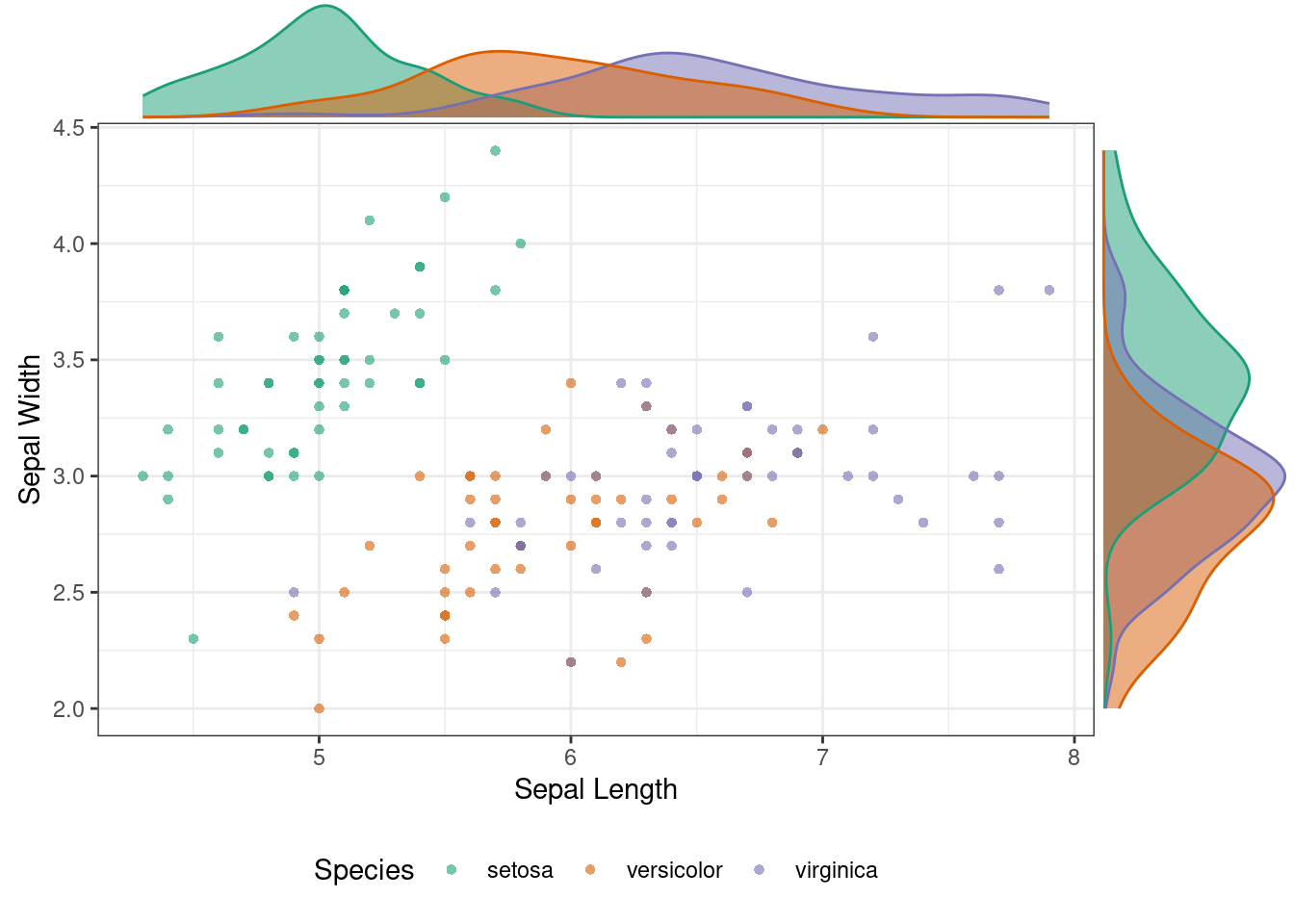 ### Plot Marginal Histogram
ggMarginal(p, type = "histogram", groupColour = TRUE, groupFill = TRUE)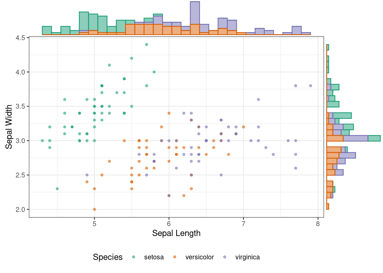 ### Plot Marginal Box Plot
ggMarginal(p, type = "boxplot", groupColour = TRUE, groupFill = TRUE)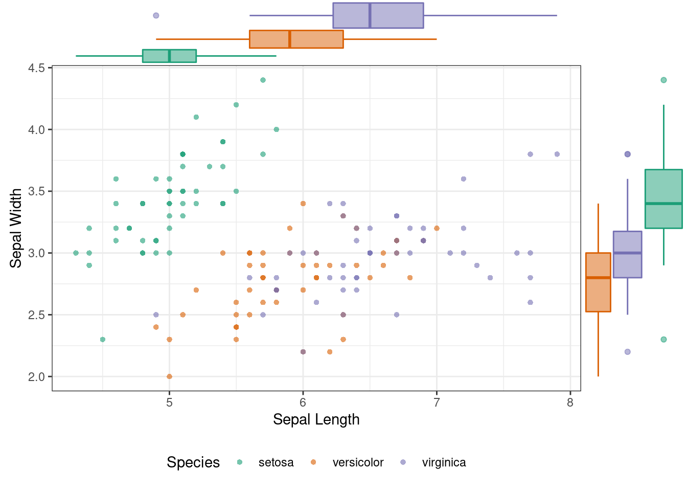
115.1.3 Plot Marginal Violin Plot
ggMarginal(p, type = "violin", groupColour = TRUE, groupFill = TRUE)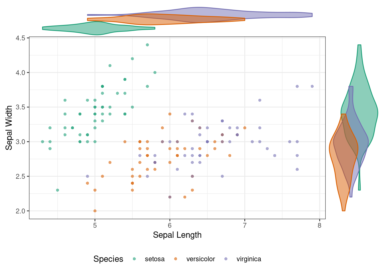 ### Plot Marginal Density Function and Histogram
ggMarginal(p, type = "densigram", groupColour = TRUE, groupFill = TRUE)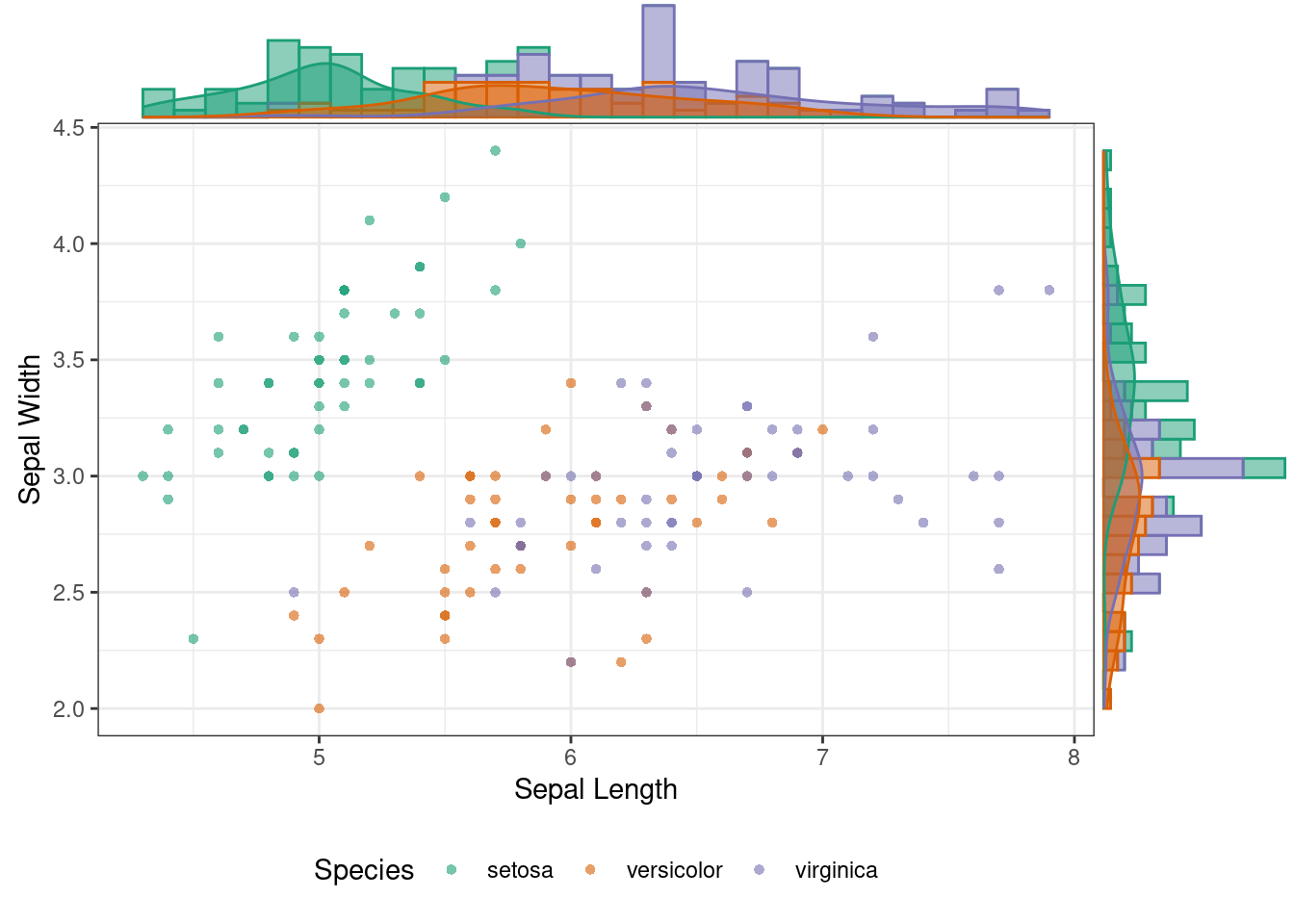
ggExtra and ggplot2 does provide some flexibility, which allows to your customise your marginal distribution. But we believe that’s not what their designer want you to do. The whole point of these libraries is to wrap up the whole complicated mechanism and let you quicklt draw a standard scatter plot with marginal distributions.
You can come up with some original designs and implement them with ggExtra and ggplot2. But believe me, it will be a unideal process. For users who like to design their own marginal distribution, we would recommend the next method.
115.2 Using cowplot and ggpubr
Same as the previous approach, let’s start with a scatter plot with no marginal distribution. Then we figure out how to add marginal distribution to it. If you want to use cowplot and ggpubr, we would recommend start your scatter plot with function ggscatter in this case, instead of ggplot.
115.2.1 Plot Another Kind of Scatter Plot
sp <- ggscatter(iris, x = "Sepal.Length", y = "Sepal.Width",
color = "Species", palette = "Accent",
size = 3, alpha = 0.6) +
border() +
theme(legend.position = "bottom")
sp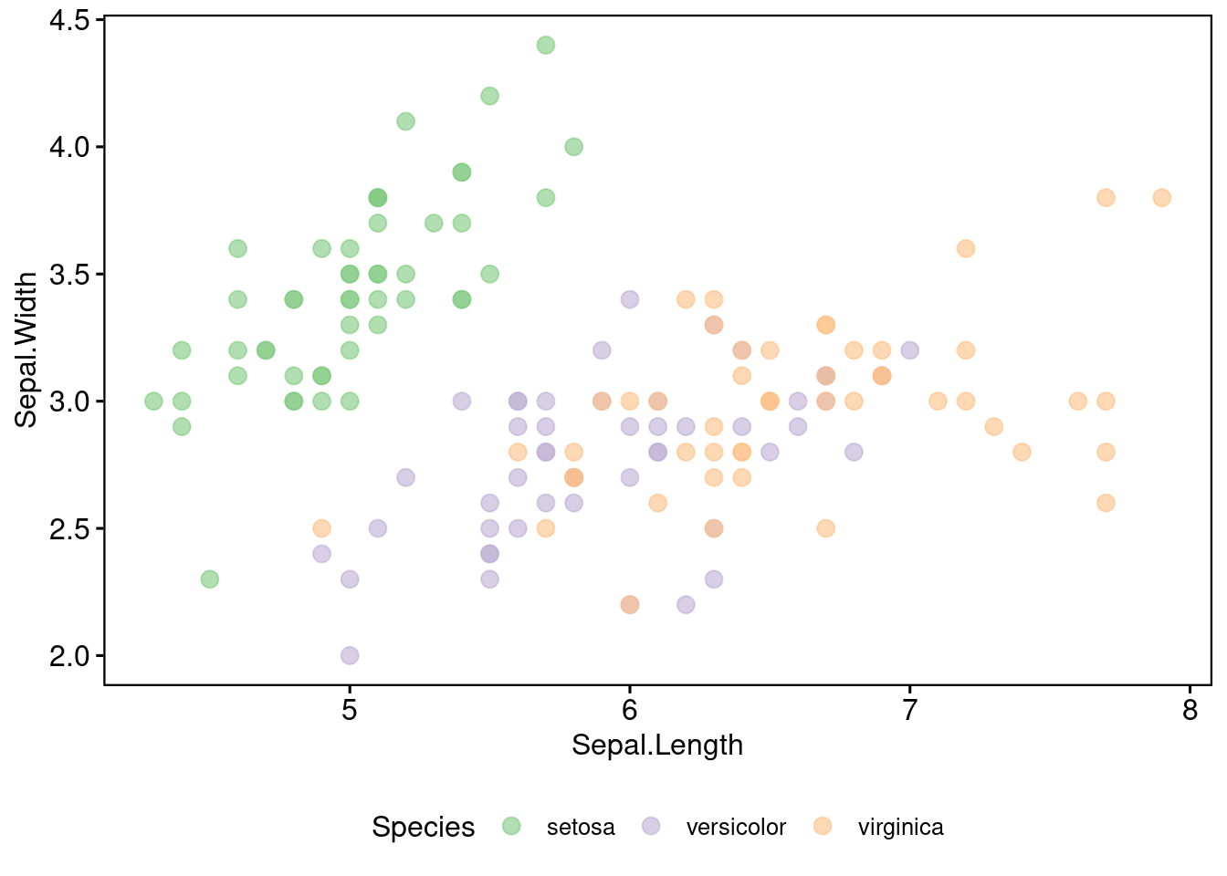 Same as before, we assign each species with a color. According colors will be shown in marginal distribution.
115.2.2 Gapped Marginal Plot
115.2.2.1 Marginal Density Plot
The process is like plotting 3 subplots: the horizontal margin, vertical margin and the scatter plot itself.
Since we already have the scatter plot, our first step is to generate the two plot: horizontal margin and vertical margin.
# Marginal density plot of x (top panel) and y (right panel)
xplot <- ggdensity(iris, "Sepal.Length", fill = "Species",
                   palette = "Accent")
yplot <- ggdensity(iris, "Sepal.Width", fill = "Species",
                   palette = "Accent") +
  rotate()
Notice that tplot is vertical because we rotate it by 90 degree. Now you can see we are really designing and customising each module by ourselves.
After that, we need to put them together using plot_grid, which you might feel familiar with. You can adjust its width, height, aligning method, and so many other options by manipulating built-in parameters of plot_grid.
# Cleaning the plots
sp <- sp + rremove("legend")
yplot <- yplot + clean_theme() + rremove("legend")
xplot <- xplot + clean_theme() + rremove("legend")
# Arranging the plot using cowplot
plot_grid(xplot, NULL, sp, yplot, ncol = 2, align = "hv",
          rel_widths = c(2, 1), rel_heights = c(1, 2))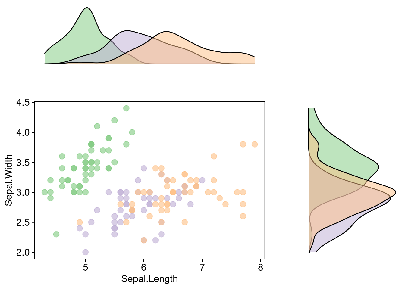
A little tip: remove the legends before puting subplots together. Legends will destroy your pretty layout.
Let’s revise the whole process, and challenge ourselves by applying the procedure to draw boxplot as marginal distribution.
115.2.2.2 Uncompressed Marginal Box Plot
# Marginal boxplot of x (top panel) and y (right panel)
xplot <- ggboxplot(iris, x = "Species", y = "Sepal.Length",
                   color = "Species", fill = "Species", palette = "Accent",
                   alpha = 0.5, ggtheme = theme_bw())+
  rotate()
yplot <- ggboxplot(iris, x = "Species", y = "Sepal.Width",
                   color = "Species", fill = "Species", palette = "Accent",
                   alpha = 0.5, ggtheme = theme_bw())
# Cleaning the plots
sp <- sp + rremove("legend")
yplot <- yplot + clean_theme() + rremove("legend")
xplot <- xplot + clean_theme() + rremove("legend")
# Arranging the plot using cowplot
plot_grid(xplot, NULL, sp, yplot, ncol = 2, align = "hv",
          rel_widths = c(2, 1), rel_heights = c(1, 2))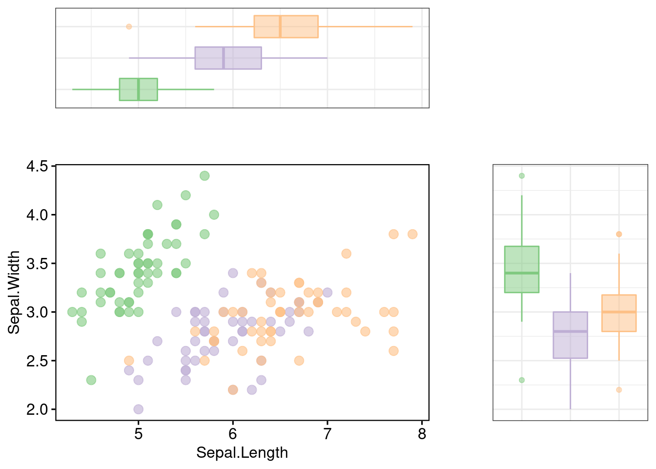
There are so many customizations you can decide during the process, that’s why cowplot and ggpubr is your idea solution for creating a original, non-standard marginal distribution. If your boss rediculously asks you to make the horizaontal margin to be a density map, and vertical margin to be a density map, now you should be confident to make that happen.
115.2.3 Connect Marginal Plot
We know some people may dislike the gaps between the scatter plot and its margin distributions. Unfortunately, if you want to get rid of it, plot_grid has to be replaced. You should use another function, axis_canvas to combine the marginal distribution with axis while creating the margin. Then, the libraries provide a really use function for you to use: insert_xaxis_grob. This function does same the job as plot_grid in the previod example.
# Main plot
pmain <- ggplot(iris, aes(x = Sepal.Length, y = Sepal.Width, color = Species)) +
  geom_point() +
  color_palette("Accent")
# Marginal densities along x axis
xdens <- axis_canvas(pmain, axis = "x") +
  geom_density(data = iris, aes(x = Sepal.Length, fill = Species),
               alpha = 0.7, size = 0.2) +
  fill_palette("Accent")
# Marginal densities along y axis
# Need to set coord_flip = TRUE, if you plan to use coord_flip()
ydens <- axis_canvas(pmain, axis = "y", coord_flip = TRUE) +
  geom_density(data = iris, aes(x = Sepal.Width, fill = Species),
               alpha = 0.7, size = 0.2) +
  coord_flip() +
  fill_palette("Accent")
p1 <- insert_xaxis_grob(pmain, xdens, grid::unit(.2, "null"), position = "top")
p2 <- insert_yaxis_grob(p1, ydens, grid::unit(.2, "null"), position = "right")
ggdraw(p2)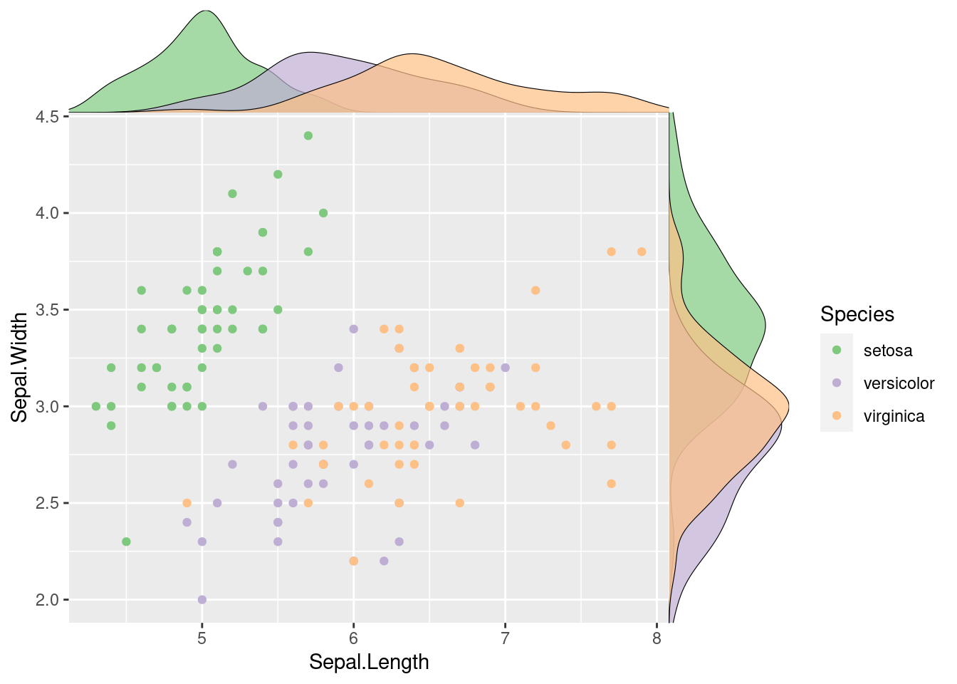
Have a clsoe at the code, you will find that it follows the same process as the previous example: creating 3 subplots and then connecting them together. This process just uses some different, yet similar functions. Similarly, you should know how to customize it.
115.3 Sources
https://cran.r-project.org/web/packages/ggExtra/index.html
https://exts.ggplot2.tidyverse.org/ggExtra.html
https://deanattali.com/2015/03/29/ggExtra-r-package/
https://cran.r-project.org/web/packages/ggExtra/vignettes/ggExtra.html