50 Dplyr tutorial in R
Pinyi Yang
#install.packages("dplyr")
#install.packages("ggplot2")
#install.packages("stringr")
library(dplyr)
library(ggplot2)
library(stringr)
50.1 Environment Setup
In order to use dyplr package, we need to first install and library it at the beginning. Besides the dplyr package, we will use two other packages for better demonstration of the functions in dplyr. Related documentations of the two accessory packages are provided below:
50.2 Introduction
Dplyr is a package of tidyverse in R. The key role of dplyr is dataframe manipulation and enables data management. Dplyr contain numerous useful functions that allows for user-friendly data query, data cleaning, data summary, etc. Dplyr is especially important for data visualization, because, an effective and informative visualization requires the structural integrity of the dataframe being used as well as the removal of excessive redundant information and keeping only the information needed.
50.3 Data
One of the most widely used data for tutorial use purpose in R is the ‘diamond’ dataset. For more information on the ‘diamond’ dataset, please visit the following link: https://www.rdocumentation.org/packages/ggplot2/versions/3.3.5/topics/diamonds.
The following section showcases the attributes of the ‘diamond’ dataset to assist the understanding of further data manipulation using dplyr.
str(diamonds)## tibble [53,940 × 10] (S3: tbl_df/tbl/data.frame)
## $ carat : num [1:53940] 0.23 0.21 0.23 0.29 0.31 0.24 0.24 0.26 0.22 0.23 ...
## $ cut : Ord.factor w/ 5 levels "Fair"<"Good"<..: 5 4 2 4 2 3 3 3 1 3 ...
## $ color : Ord.factor w/ 7 levels "D"<"E"<"F"<"G"<..: 2 2 2 6 7 7 6 5 2 5 ...
## $ clarity: Ord.factor w/ 8 levels "I1"<"SI2"<"SI1"<..: 2 3 5 4 2 6 7 3 4 5 ...
## $ depth : num [1:53940] 61.5 59.8 56.9 62.4 63.3 62.8 62.3 61.9 65.1 59.4 ...
## $ table : num [1:53940] 55 61 65 58 58 57 57 55 61 61 ...
## $ price : int [1:53940] 326 326 327 334 335 336 336 337 337 338 ...
## $ x : num [1:53940] 3.95 3.89 4.05 4.2 4.34 3.94 3.95 4.07 3.87 4 ...
## $ y : num [1:53940] 3.98 3.84 4.07 4.23 4.35 3.96 3.98 4.11 3.78 4.05 ...
## $ z : num [1:53940] 2.43 2.31 2.31 2.63 2.75 2.48 2.47 2.53 2.49 2.39 ...
head(diamonds, n = 3)## # A tibble: 3 × 10
## carat cut color clarity depth table price x y z
## <dbl> <ord> <ord> <ord> <dbl> <dbl> <int> <dbl> <dbl> <dbl>
## 1 0.23 Ideal E SI2 61.5 55 326 3.95 3.98 2.43
## 2 0.21 Premium E SI1 59.8 61 326 3.89 3.84 2.31
## 3 0.23 Good E VS1 56.9 65 327 4.05 4.07 2.31## carat depth table price
## Min. :0.2000 Min. :43.00 Min. :43.00 Min. : 326
## 1st Qu.:0.4000 1st Qu.:61.00 1st Qu.:56.00 1st Qu.: 950
## Median :0.7000 Median :61.80 Median :57.00 Median : 2401
## Mean :0.7979 Mean :61.75 Mean :57.46 Mean : 3933
## 3rd Qu.:1.0400 3rd Qu.:62.50 3rd Qu.:59.00 3rd Qu.: 5324
## Max. :5.0100 Max. :79.00 Max. :95.00 Max. :18823
## x y z
## Min. : 0.000 Min. : 0.000 Min. : 0.000
## 1st Qu.: 4.710 1st Qu.: 4.720 1st Qu.: 2.910
## Median : 5.700 Median : 5.710 Median : 3.530
## Mean : 5.731 Mean : 5.735 Mean : 3.539
## 3rd Qu.: 6.540 3rd Qu.: 6.540 3rd Qu.: 4.040
## Max. :10.740 Max. :58.900 Max. :31.80050.4 Column and Row Manipulation
In data analysis, sometimes the original data set contains too much information, more than what we actually need for further analysis or it does not have a good structure for us to use. In order to make the data looked structured, we would use Dplyr to organize and clean Data. Dplyr can effectively help us reorganize the data set based on criteria we commanded. For example, the data set may contain all observations (i.e. rows) from the past 10 years, while we only need to analyze the trend in the recent 5 years. In this case, we need to ignore the data from the previous years in order to generate reasonable visualizations, thus the filter function in Dplyr will come in handy. Also, there might be times when the data contains numerous redundant parameters (i.e. columns) for analysis, and we need to only select those variables that are important for the goal of the study. In this case, we can use Dplyr’s select function to choose desired columns. ### Select The ‘select’ in dplyr package is used to select certain columns from the data frame. We can use the ‘select’ function with the following syntax: \[select(data, column\ names/column\ position , \dots)\] #### Column Selection In the following example, we are selecting three columns of observations only: ‘carat’, ‘clarity’, and ‘price’. Noted here that we can select by its name or by its position.
#only keeping "carat", "clarity", and "price" columns
select_result <- select(diamonds, c(carat, clarity, price))
head(select_result,n = 3)## # A tibble: 3 × 3
## carat clarity price
## <dbl> <ord> <int>
## 1 0.23 SI2 326
## 2 0.21 SI1 326
## 3 0.23 VS1 327
# same result but use position
select_result <- select(diamonds, c(1,4,7))
head(select_result,n = 3)## # A tibble: 3 × 3
## carat clarity price
## <dbl> <ord> <int>
## 1 0.23 SI2 326
## 2 0.21 SI1 326
## 3 0.23 VS1 327
# or use both column name and position, not recommended
select_result <- select(diamonds, c(1,4, price))
head(select_result,n = 3)## # A tibble: 3 × 3
## carat clarity price
## <dbl> <ord> <int>
## 1 0.23 SI2 326
## 2 0.21 SI1 326
## 3 0.23 VS1 32750.4.0.1 Column Deselection
We can also deselect certain columns, or a range of columns using the negate command \(!\). In the following example, we want to remove (i.e. deselect) columns from x to z.
#deselecting columns from x to z
select_result <- select(diamonds, !(x:z))
head(select_result,n = 3)## # A tibble: 3 × 7
## carat cut color clarity depth table price
## <dbl> <ord> <ord> <ord> <dbl> <dbl> <int>
## 1 0.23 Ideal E SI2 61.5 55 326
## 2 0.21 Premium E SI1 59.8 61 326
## 3 0.23 Good E VS1 56.9 65 32750.4.0.2 Helper Functions
there are several helper functions for selection that deal with specific cases to be used with select function:
\(contains()\): Use it to select column which contains a specific string
\(starts\_with()\): Use it to select columns which start with given string
\(ends\_with()\): Use it to select columns which end with given string
\(matches()\): Use it to select columns that match a string (often use regular expression)
\(everything()\): Select all columns
50.4.0.3 The matches() Function
As introduced above, the \(matches()\) function can select columns with names that match a regular expression (regex). Regular expression is a way to represent certain string patterns, which is extensively used in natural language processing, linguistic analysis, etc. For details in regular expression, such as grammar, and its application, please visit the following link: https://developer.mozilla.org/en-US/docs/Web/JavaScript/Guide/Regular_Expressions/Cheatsheet.
For example, if we only want to keep columns with names that start with c, we can use the regular expression of “^c” in the \(matches()\) function. (p.s. “^c” is a regular expression that defines strings that start with the letter lower-case c)
## # A tibble: 3 × 4
## carat cut color clarity
## <dbl> <ord> <ord> <ord>
## 1 0.23 Ideal E SI2
## 2 0.21 Premium E SI1
## 3 0.23 Good E VS1Notice that only the columns “carat”, “cut”, “color”, and “clarity” are kept after selection, because they all satisfy the pattern that the first letter of the string is the letter “c”.
50.4.0.4 The contains() Function
For the sake of demonstration, we will create a pseudo-dataset with names specifically designed to include certain strings. In this case, multiple column names include the string “length”
colors <- c("red", "blue", "yellow", "green")
pseudo_car_data <- data.frame(obs = 1:10,
cabin_length = runif(10, 5, 7.5),
door_length = runif(10, 1, 3),
wind_shield_length = runif(10, 4, 6),
color = sample(colors, 10, replace = T))
head(pseudo_car_data,,n = 3)## obs cabin_length door_length wind_shield_length color
## 1 1 6.274862 1.146336 5.500834 green
## 2 2 5.153703 1.517312 4.992886 red
## 3 3 7.241021 1.917732 5.349165 blueNow, we can use the \(contains()\) function to select those names that contain the string “length”.
## cabin_length door_length wind_shield_length
## 1 6.274862 1.146336 5.500834
## 2 5.153703 1.517312 4.992886
## 3 7.241021 1.917732 5.34916550.4.1 Filter
Similar to the select function that we discussed in the last section, the filter function in dplyr package is also used for selection from the existing data frame. Filter function is used to select rows that satisfies specific conditions/criteria.The second argument here must be logical value. Logical operation would be useful here. For example, the ‘is.na’ function would return TRUE if a value is NA and FALSE if it is not. We can also use \(\&\) and \(|\) operators to combine multiple logical statements.
The syntax for the filter function is as follow: \[filter(data, condition, \dots)\]
50.4.1.1 Filter Numerical Values
The filter function can be used to filter both numerical and character type data. First, lets use the price parameter to demonstrate how to filter numerical values. We will filter out the observations that have diamond price over 500. In other words, we will only keep those rows of observations with \(price \leq 500\).
#the range of prices for diamonds
range(diamonds$price)## [1] 326 18823
#filter observations that have price less than or equal to 500
filter_result <- filter(diamonds, price <= 500)
head(filter_result,n = 3)## # A tibble: 3 × 10
## carat cut color clarity depth table price x y z
## <dbl> <ord> <ord> <ord> <dbl> <dbl> <int> <dbl> <dbl> <dbl>
## 1 0.23 Ideal E SI2 61.5 55 326 3.95 3.98 2.43
## 2 0.21 Premium E SI1 59.8 61 326 3.89 3.84 2.31
## 3 0.23 Good E VS1 56.9 65 327 4.05 4.07 2.3150.4.1.2 Filter Character Values
Now, we can filter by character type variables. For example, we can choose those observations that have “Fair” or “Good” cuts:
#check levels of cuts
levels(diamonds$cut)## [1] "Fair" "Good" "Very Good" "Premium" "Ideal"
table(diamonds$cut)##
## Fair Good Very Good Premium Ideal
## 1610 4906 12082 13791 21551
#filter by cut, keeping Fair and Good
filter_result <- filter(diamonds, cut %in% c("Fair", "Good"))
head(filter_result,n = 3)## # A tibble: 3 × 10
## carat cut color clarity depth table price x y z
## <dbl> <ord> <ord> <ord> <dbl> <dbl> <int> <dbl> <dbl> <dbl>
## 1 0.23 Good E VS1 56.9 65 327 4.05 4.07 2.31
## 2 0.31 Good J SI2 63.3 58 335 4.34 4.35 2.75
## 3 0.22 Fair E VS2 65.1 61 337 3.87 3.78 2.49
table(filter_result$cut)##
## Fair Good Very Good Premium Ideal
## 1610 4906 0 0 0By checking the counts of each category, we can see that after filtering the dataframe, all observations with cut being “Very Good” or “Premium” or “Ideal” are filtered out, leaving only “Fair” or “Good” observations. Note that the table after filtration still contains the other three categories. This is because the ‘cut’ variable is stored as a factor in the dataframe. Thus, filtration will not eliminate all the original levels.
50.4.2 Slice
The slice function in dplyr is also useful for selecting rows based on its position or order. The use of it is similar to head function in base R which would select the top or tail n rows in the data set.
The syntax for the slice function is as follow: \[slice(data, number\ to\ be\ sliced,... )\]
#only get the first five observation of the data frame
slice_result <- slice(diamonds, 1:5)
slice_result ## # A tibble: 5 × 10
## carat cut color clarity depth table price x y z
## <dbl> <ord> <ord> <ord> <dbl> <dbl> <int> <dbl> <dbl> <dbl>
## 1 0.23 Ideal E SI2 61.5 55 326 3.95 3.98 2.43
## 2 0.21 Premium E SI1 59.8 61 326 3.89 3.84 2.31
## 3 0.23 Good E VS1 56.9 65 327 4.05 4.07 2.31
## 4 0.29 Premium I VS2 62.4 58 334 4.2 4.23 2.63
## 5 0.31 Good J SI2 63.3 58 335 4.34 4.35 2.75There are also other wrapper functions for ‘slice’ that can be used to get the pieces of data with specified number/range of rows while also filtering with some conditions, such as slice_max,slice_min. The syntax for the slice function is as follow: \[slice\_max(data, order\_by = column \ name, n = number\ to\ be\ sliced )\]
# only get the first five observation of the data frame with highest price
slice_result <- slice_max(diamonds, order_by = price, n = 5)
slice_result## # A tibble: 5 × 10
## carat cut color clarity depth table price x y z
## <dbl> <ord> <ord> <ord> <dbl> <dbl> <int> <dbl> <dbl> <dbl>
## 1 2.29 Premium I VS2 60.8 60 18823 8.5 8.47 5.16
## 2 2 Very Good G SI1 63.5 56 18818 7.9 7.97 5.04
## 3 1.51 Ideal G IF 61.7 55 18806 7.37 7.41 4.56
## 4 2.07 Ideal G SI2 62.5 55 18804 8.2 8.13 5.11
## 5 2 Very Good H SI1 62.8 57 18803 7.95 8 5.0150.5 Order Manipulation
Sometimes, we want to get a direct visualization of the data by ranking the observations using one or multiple parameters. ### Ascending Order We can use the ‘arrange’ function to arrange data, based on one parameter or multiple parameters, in an ascending order, using the following syntax: \[arrange(data, column\ for\ arrangement, \dots)\]
## # A tibble: 3 × 10
##   carat cut     color clarity depth table price     x     y     z
##   <dbl> <ord>   <ord> <ord>   <dbl> <dbl> <int> <dbl> <dbl> <dbl>
## 1  0.23 Ideal   E     SI2      61.5    55   326  3.95  3.98  2.43
## 2  0.21 Premium E     SI1      59.8    61   326  3.89  3.84  2.31
## 3 0.23 Good E VS1 56.9 65 327 4.05 4.07 2.3150.5.1 Descending Order
We can use the ‘desc’ function to arrange data, based on one or multiple parameters, in a descending order, using the following syntax: \[arrange(data, desc(column\ for\ arrangement))\]
## # A tibble: 3 × 10
##   carat cut       color clarity depth table price     x     y     z
##   <dbl> <ord>     <ord> <ord>   <dbl> <dbl> <int> <dbl> <dbl> <dbl>
## 1  2.29 Premium   I     VS2      60.8    60 18823  8.5   8.47  5.16
## 2  2    Very Good G     SI1      63.5    56 18818  7.9   7.97  5.04
## 3  1.51 Ideal     G     IF       61.7    55 18806  7.37  7.41  4.56
50.6 Entry Manipulation
In real life data processing, sometimes, we need to gather data in order to reduce the dimension. For example, if we want to show the mean of number of products sold across all months while the data shows daily sales. In this case, we need to gather observations by combining observations within the same month and calculate their cumulative mean and generate the desirable visualizations. This is when the grouping function and summary function in dplyr comes in handy. ### Grouping Grouping function in dplyr groups data based on the categories in the assigned column(s). The general syntax is: \[group\_by(data, column\ used\ for\ grouping, \dots)\]
## # A tibble: 3 × 10
## # Groups:   cut [3]
##   carat cut     color clarity depth table price     x     y     z
##   <dbl> <ord>   <ord> <ord>   <dbl> <dbl> <int> <dbl> <dbl> <dbl>
## 1  0.23 Ideal   E     SI2      61.5    55   326  3.95  3.98  2.43
## 2  0.21 Premium E     SI1      59.8    61   326  3.89  3.84  2.31
## 3  0.23 Good    E     VS1      56.9    65   327  4.05  4.07  2.31
head(diamonds,n = 3)## # A tibble: 3 × 10
## carat cut color clarity depth table price x y z
## <dbl> <ord> <ord> <ord> <dbl> <dbl> <int> <dbl> <dbl> <dbl>
## 1 0.23 Ideal E SI2 61.5 55 326 3.95 3.98 2.43
## 2 0.21 Premium E SI1 59.8 61 326 3.89 3.84 2.31
## 3 0.23 Good E VS1 56.9 65 327 4.05 4.07 2.31Notice that the dataframe before and after grouping looks exactly the same! This is because the ‘group_by’ function does not change the dataframe itself, rather, it prepares the dataframe for further data processing. As we can see in the next section, we can summarize the data after grouping.
50.6.1 Summary Statistics
Often times, we want to reduce the complexity of the data by creating summary statistics, such as the mean, median, max, etc. The ‘summarise’ function in dplyr do just the job. After grouping by categories in certain column(s), we can employ the ‘summarise’ function to create new column(s) of summary statistics, with the following syntax: \[summarise(grouped\_data, new\_column\_name = function(column\ to\ be\ summarized), \dots)\]
For example, here we are trying to get the mean price based on the cut of diamond type.
## # A tibble: 5 × 2
##   cut       mean_price
##   <ord>          <dbl>
## 1 Fair           4359.
## 2 Good           3929.
## 3 Very Good      3982.
## 4 Premium        4584.
## 5 Ideal 3458.50.6.2 Mutation
The ‘mutate’ function is extremely useful for data manipulation not only because it allows for greater freedom in transforming the existing dataframe, but also because of its application in missing value imputation. The syntax for the mutate function is: \[mutate(data, new\_column\_name = operation, \dots)\]
50.6.2.1 Transforming Dataframe
We can add a new parameter by performing operations on existing parameters. In the following example, we will calculate the price per carat diamond for each diamond listed in the dataset. To do so we can use the formula \(\frac{price}{carat}\) for each row of observation.
## # A tibble: 3 × 11
## carat cut color clarity depth table price x y z price_per_ca…¹
## <dbl> <ord> <ord> <ord> <dbl> <dbl> <int> <dbl> <dbl> <dbl> <dbl>
## 1 0.23 Ideal E SI2 61.5 55 326 3.95 3.98 2.43 1417.
## 2 0.21 Premium E SI1 59.8 61 326 3.89 3.84 2.31 1552.
## 3 0.23 Good E VS1 56.9 65 327 4.05 4.07 2.31 1422.
## # … with abbreviated variable name ¹price_per_caratNotice that the mutated dataframe has one more column at the end titled “price_per_carat”. The new column is calculated by dividing price by carat within each observation.
50.6.2.2 Imputation – Using Mean
For the sake of demonstration, we will create a pseudo-dataset that contains missing values to showcase the imputation power of the mutate function.
#create new data
pseudo_missing_data <- data.frame(name = c("Tom", "Jay", "Marry", "Lexa", "Garcia"),
                          age = c(sample(40:80, 3, replace = F), NA, NA))
pseudo_missing_data
## name age
## 1 Tom 56
## 2 Jay 57
## 3 Marry 62
## 4 Lexa NA
## 5 Garcia NAIn the example, we can see that Lexa and Garcia’s ages are missing. We will use mutate function to impute the missing values by using the mean of the rest of the ages (i.e. age of Tom, Jay, and Marry). The \(is.na()\) function is used to check if the entry contain NA values.
imputed_data <- mutate(pseudo_missing_data,
                       age = ifelse(is.na(age), mean(age, na.rm = T), age))
imputed_data
## name age
## 1 Tom 56.00000
## 2 Jay 57.00000
## 3 Marry 62.00000
## 4 Lexa 58.33333
## 5 Garcia 58.3333350.6.2.3 Imputation – Removing Observations
Also, there is a more brutal way of cleaning the data – removing observations with NA values (i.e. removing the entire row if that row contain NA value). However, this type of cleaning technique is generally not recommended when there are large quantity of missing values, because it will severely depricate the integrity of the original dataset and lose important information. But the general way of removing observations with NA values is by calling the ‘na.omit’ function:
na.omit(pseudo_missing_data)## name age
## 1 Tom 56
## 2 Jay 57
## 3 Marry 62We can see that the latter two rows (i.e. observations of Lexa and Garcia) are completely removed!
50.6.2.4 Useful Helper Functions for mutate()
There are multiple functions that can be embedded in the ‘mutate’ function which helps perform complex tasks that otherwise requires us to define functions by ourselves:
\(pmin(), pmax()\): Element-wise min and max
\(cummin(), cummax()\): Cumulative min and max
\(between()\): If the value is in a range
\(cumsum(), cumprod()\): Cumulative sum and cumulative product
\(cummean()\): Cumulative mean
example:
helper_example <- mutate(diamonds,
                         #use cummin to find the minimum value up to the current observation
                         cummin_price = cummin(price),
                         #use between to determine if the price is in range
                         in_range = between(price, 330, 340))
head(helper_example)[,c("price", "cummin_price", "in_range")]
## # A tibble: 6 × 3
## price cummin_price in_range
## <int> <int> <lgl>
## 1 326 326 FALSE
## 2 326 326 FALSE
## 3 327 326 FALSE
## 4 334 326 TRUE
## 5 335 326 TRUE
## 6 336 326 TRUE50.6.3 Distinct
The ‘distinct’ function is used to check if there is any duplicates in the data set. Because we wouldn’t want our data to have excessive duplicated observations. The distinct function can help us to delete the replicated rows and simplify the dataframe. \[distinct(data, \dots)\]
repeated_diamonds <- slice(diamonds,1:3,1:2)
repeated_diamonds
## # A tibble: 5 × 10
## carat cut color clarity depth table price x y z
## <dbl> <ord> <ord> <ord> <dbl> <dbl> <int> <dbl> <dbl> <dbl>
## 1 0.23 Ideal E SI2 61.5 55 326 3.95 3.98 2.43
## 2 0.21 Premium E SI1 59.8 61 326 3.89 3.84 2.31
## 3 0.23 Good E VS1 56.9 65 327 4.05 4.07 2.31
## 4 0.23 Ideal E SI2 61.5 55 326 3.95 3.98 2.43
## 5 0.21 Premium E SI1 59.8 61 326 3.89 3.84 2.31
distinct(repeated_diamonds )## # A tibble: 3 × 10
## carat cut color clarity depth table price x y z
## <dbl> <ord> <ord> <ord> <dbl> <dbl> <int> <dbl> <dbl> <dbl>
## 1 0.23 Ideal E SI2 61.5 55 326 3.95 3.98 2.43
## 2 0.21 Premium E SI1 59.8 61 326 3.89 3.84 2.31
## 3 0.23 Good E VS1 56.9 65 327 4.05 4.07 2.3150.7 Piping - Tying Everything Together
Piping is an effective way to construct data processing pipelines, especially when the process involves multiple manipulation steps. The grammar used to pipe down commands is the ‘%>%’. The direction where the arrow is pointing towards is the way that data processing proceeds.
For example, we want to first filter out the observations that have ‘Good’ cut; then only keep the parameters that are numerical (i.e. ‘carat’, ‘price’, ‘depth’, ‘table’, ‘x’, ‘y’, ‘z’), as well as ‘clarity’; then, summarize the data by taking the mean of price grouping by ‘clarity’.
#pass down to the next manipulation command using piping
diamonds %>%
  #filter only those observations with Good cuts
  filter(cut == "Good") %>%
  #select all columns except for cut and color
  select(-c(cut, color)) %>%
  #summarize the price when grouping by clarity
  group_by(clarity) %>%
  summarise(mean_price = mean(price)) %>%
  #order the mean prices in descending order of clarity
  arrange(desc(mean_price))
## # A tibble: 8 × 2
## clarity mean_price
## <ord> <dbl>
## 1 SI2 4580.
## 2 VS2 4262.
## 3 IF 4098.
## 4 VS1 3801.
## 5 SI1 3690.
## 6 I1 3597.
## 7 VVS2 3079.
## 8 VVS1 2255.be careful when using piping with ggplot2. We know from ggplot2 that different layers of graphical components are connected by \(+\) sign. Even though the piping operator \(%>%\) has the same function as the plus sign, they are used under different conditions. Don’t mix them up!
50.8 Using Dplyr with GGplot
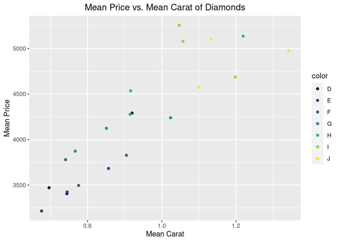
The essence of dplyr is to clean the data before it is used to perform model construction or data visualization. In this section, we will use a simple data visualization example that combines dplyr and ggplot2 and shows how we can tie the functions we have introduced above with graphic design using ggplot2.
diamonds %>%
  #data manipulation using dplyr
  filter(cut %in% c("Fair", "Good", "Very Good")) %>%
  select(cut, carat, color, price) %>%
  group_by(cut, color) %>%
  summarise(mean_price = mean(price),
            mean_carat = mean(carat)) %>%
  #data visualization using ggplot2
  ggplot(mapping = aes(x = mean_carat, y = mean_price)) +
  geom_point(mapping = aes(color = color)) +
  ylab("Mean Price") + xlab("Mean Carat") +
  labs(title = "Mean Price vs. Mean Carat of Diamonds") +
  theme(plot.title = element_text(hjust = 0.5))