108 Improved density estimation
Abel Perez Vargas
108.1 Introduction
In the field of data analysis it is common to come across non-negative variables, such as waiting times, prices, distances, age and weight, as well as non-positive variables such as money due, level below the sea or below freezing point temperature.
Before thinking in further modeling of such variables, we may be first interested in exploring and visualizing the data. And among the first techniques one may want to implement, there is univariate visualization.
Density plots are a very useful technique that unveils the distributional form of the variables, and it may help us identify patterns that may be hidden in a traditional histogram (e.g. “gaps” in the data that may happen to be inside one specific histogram class).
However, density plots may sometimes give the false impression that a know-to-be non-negative variable has some negative values like in this example using simulations of a \(\Gamma(2,2)\) distribution.
set.seed(123)
plot(density(rgamma(100, 2, 2) ), lty=2, lwd=2, col="red", main="Densities")
curve(dgamma(x, 2, 2), from=-1, to=5, lwd=2, add=T)
legend("topright", legend=c("True density", "Estimated density"),
       lty=c(1, 2), col=c("black", "red"))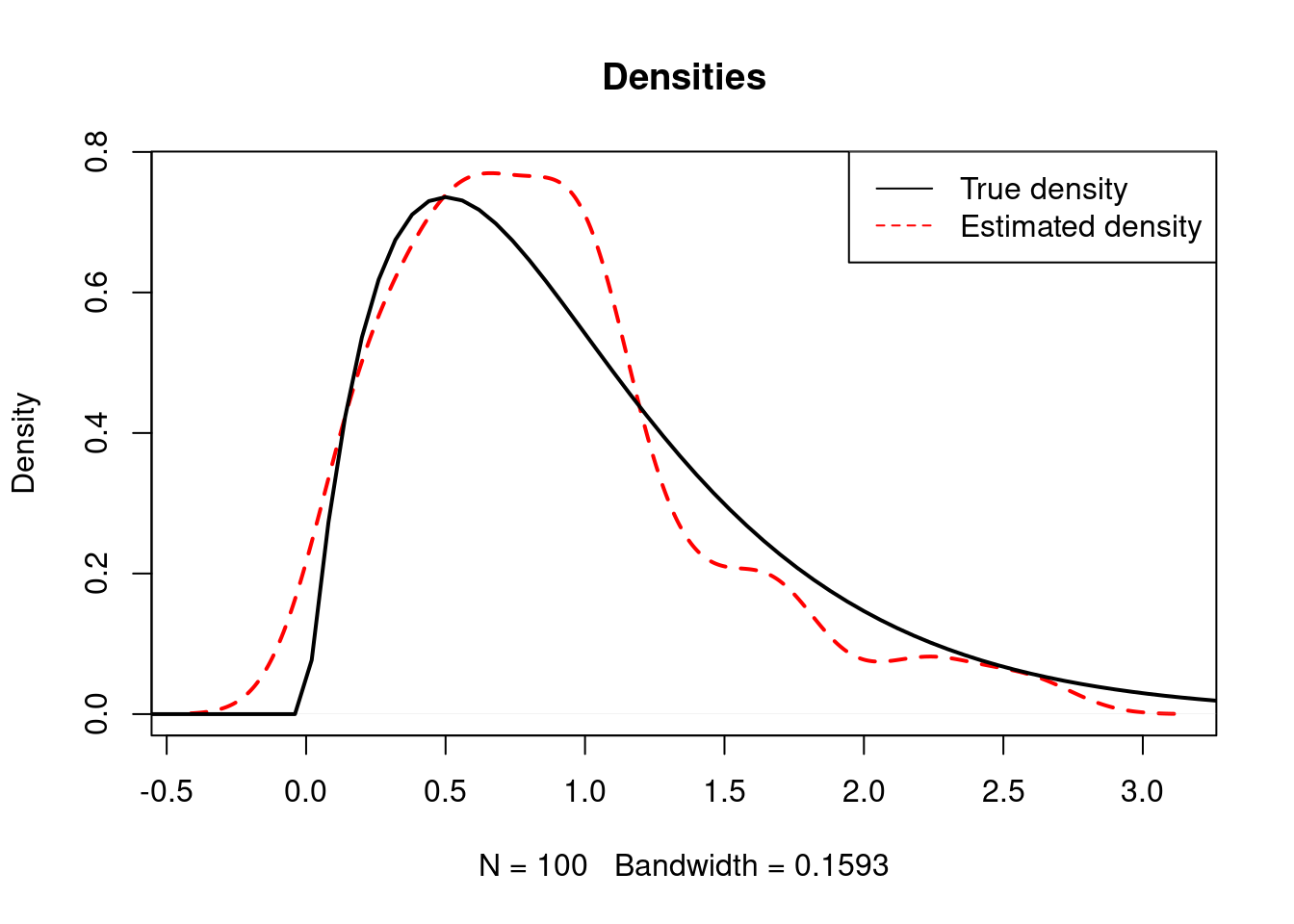
It can also be the case that the data exhibits values exactly equal to 0, in which case the standard density plot cannot help us detect it and we would have to do further exploration in order to do it.
set.seed(123)
data <- c(rep(0, 10), rgamma(100, 1, 1))
plot(density( data ), lty=2, lwd=2, col="red",  main="Densities")
legend("topright", legend="Estimated density",
       lty=2, col="red")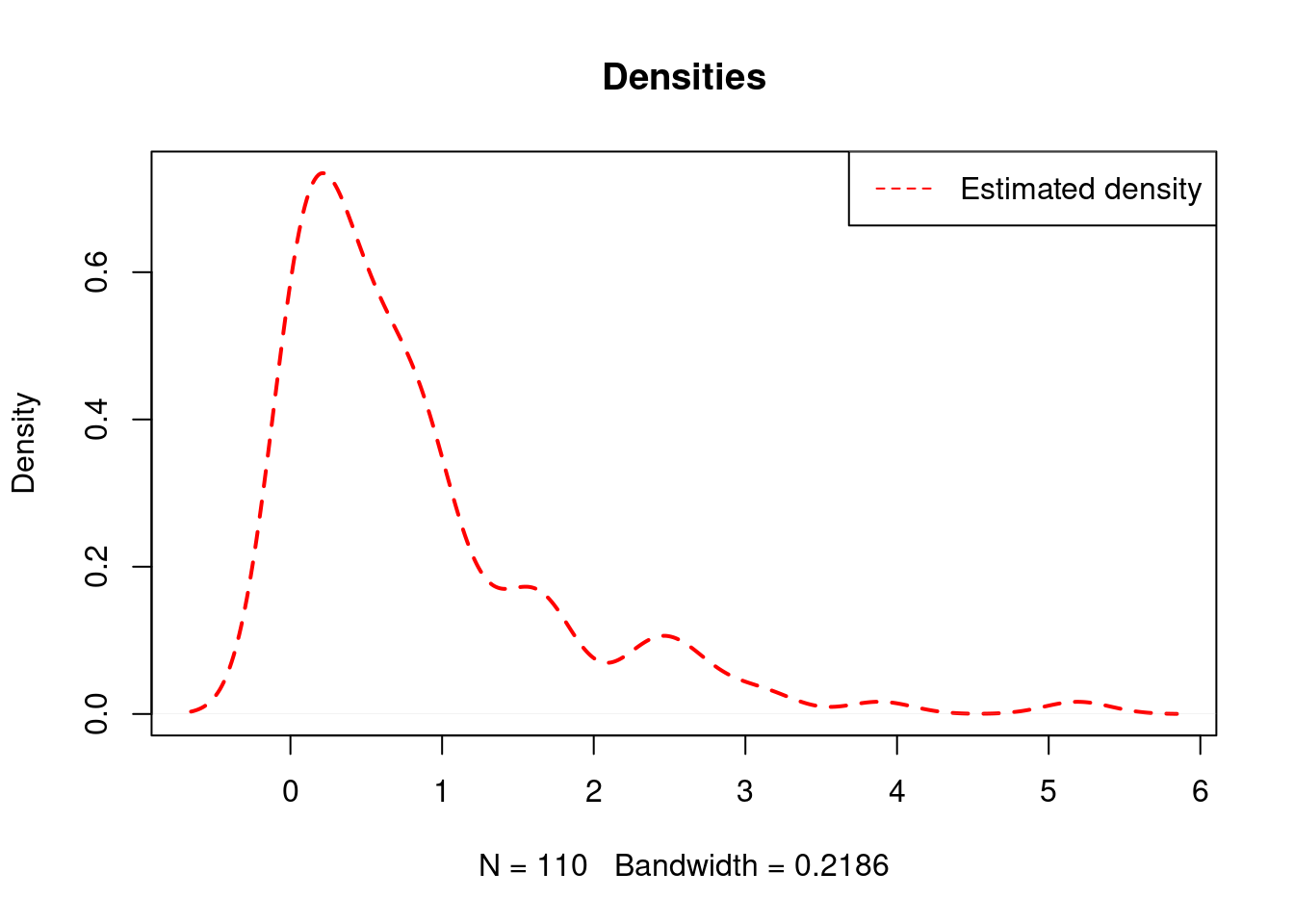
## [1] "Frequency of 0: 10"108.2 Generalizing Kernel Smoothing for Densities
In this tutorial we focus on density plots, or more formally, density estimation based on kernels (Venables & Ripley, 2002) for data that may come from a mixture of discrete and continuous random variables (e.g. data exhibiting 0’s), and avoid positive density below or above 0 if the data exhibits such behavior.
For this, we first perform an algorithm that detects repeated values in the data and then tests their significance with a Binomial test for the proportion with the following hypothesis: \[H_0: p_i=\frac{1}{n} ~~ vs ~~ H_1: p_i>\frac{1}{n},\] for \(i\) an index for such values with repetitions.
If repeated values are found to be statistically significant (that is, when \(H_0\) is rejected under \(\alpha=0.05\)), we then model the data as a mixture of a discrete random variable with support on the repeated values, and a continuous random variable for the data without repetitions, which implies the following density: \[ f_X(x)=\sum_{i^*}\hat{p}_{i^*} \delta_{ \{ x_{i^*} \} }(x) ~ + ~ \left( 1-\sum_{i^*}\hat{p}_{i^*} \right)g(x),\] where \(g\) is the density estimate of the data without the significant repeated values: \(x_{i^*}\), \(\hat{p}_{i^*}\) represents the estimated probability mass (proportion) of such values, and \(\delta_{ \{ k \}}(x)\) is Dirac’s delta, a function that is equal to infinity in \(k\), \(0\) otherwise, and integrates to one.
The previous representation is useful to keep \(f_X\) as a valid density function, but for visualization purposes we will only plot \(\hat{p}_{i^*}\) as Dirac’s delta would be represented as a vertical infinite line.
The density \(g\) will be modified from the standard stats::density function in R to avoid positive density in non-admissible regions (like in the negative numbers if all the data are all positive). For that end, we will slightly modify the kernel method of density estimation, by generalizing the gaussian kernel to truncated normal for the smoothing. In the case of non-negative data, the kernel will be truncated to be distinct than \(0\) only for \(x\geq0\) (and a similar case for non-positive data).
108.3 plot_density Function
We introduce plot_density, a function that adjusts itself in the presence of non-negative, non-positive or real data to avoid assigning density to unlikely values, and also automatically detects the presence of significant repeated values in the data.
# plot_density function
#
# Inputs:
#
# x: data, a numeric vector possibly with repeated values
# k: split parameter (default=0), the value for which the function will
#    evaluate whether or not the data is all "to the left", "to the right"
#    or neither from k
# bw: bandwidth, either the character "nrd0" as in stats::density, or a number
#     for manual bandwidth selection
# main, xlab, ylab: graphical parameters to be passed to base::plot
#
# Output: data density plot with displayed relative frequency of repeated vales (if that's the case)
plot_density <- function(x, thr=0, bw="nrd0",
                         main="Density Plot", xlab="x", ylab="density"){

  if(sum(is.na(x))>0 ){
    stop("NAs found")
  }else{

    # Repeated Values detection

    n <- length(x)
    x <- sort(x)
    y <- x[-1][x[-1]==x[-n]]
    vals <- NULL

    # Smallest difference distinct than 0 to be used for plot margins
    diff <- x[-1]-x[-n]
    diff <- min(diff[diff>0])

    if(length(y)>0 ){
      rep <- table(y) + 1# frequency of the repeated values
      M <- sapply(rep, binom.test, n=n, p=1/n,
             alternative="greater")# binomial test p-values
      M <- unlist(M[row.names(M)=="p.value", ])

      vals <- names(rep)[M<0.05]
      freq <- rep[M<0.05]

      # If significant values where detected, they are stored in 'vals'
      if(length(vals)>0){
        vals <- as.numeric(vals)
      }
    }

    # banwidth

    if(bw=="nrd0"){
      # Silverman's rule of thumb: Silverman (1986, page 48, eqn (3.31)))
      IQ <- quantile(x, 0.75) - quantile(x, 0.25)
      if(IQ>0){
        bw <- 0.9*min((sd(x)/1.34*n)^(-1/5), (IQ/1.34*n)^(-1/5))
      }else{
        bw <- 0.9*(sd(x)/1.34*n)^(-1/5)
      }

    }


    # Density plotting


    if( min(x)>=thr ){
      # Non-negative case: Gaussian kernel modified to positive truncated Normal


      # Truncated normal kernel
      k <- function(x, m, sd){
        if(x<0){
          0
        }else{
          dnorm(x, m, sd)/(1-pnorm(0, m, sd))
        }
      }


      if(length(y)>0 & length(vals)>0){
        # Discrete probability mass will be plotted

        p <- freq/n# mass probabilities
        c <- x[!x %in% vals]# continuous component

        # continous density component re-scaled with the mass probability
        d <- function(x, c, bw){
          (1-sum(p))*mean(k(x, c, bw))
        }

        # Plot
        grid <- c( min(x)-diff, c, max(x)+diff )
        plot(grid, sapply( grid, d, c, bw ), main=main, xlab=xlab,
             ylab=ylab, col="darkgray", type="l")
        points(vals, p, pch=16)
        for(j in 1:length(vals)){lines(c(vals[j], vals[j]), c(0, p[j]) )}
        legend("topright", legend="Mass Probability", col="black", pch=16)

      }else{
        # No probability mass found

        # continous density
        d <- function(x, c, bw){
          mean(k(x, c, bw))
        }

        # Plot
        grid <- c( min(x)-diff, x, max(x)+diff )
        plot(grid, sapply( grid, d, x, bw ), main=main, xlab=xlab,
             ylab=ylab, col="gray", type="l")

      }


    }else{


      if( max(x)<=thr ){
        # Non-positive case: Gaussian kernel modified to negative truncated Normal

        # Truncated normal kernel
        k <- function(x, m, sd){
          if(x>0){
            0
          }else{
            dnorm(x, m, sd)/pnorm(0, m, sd)
          }
        }


        if(length(y)>0 & length(vals)>0){
          # Discrete probability mass will be plotted

          p <- freq/n# mass probabilities
          c <- x[!x %in% vals]# continuous component

          # continous density component re-scaled with the mass probability
          d <- function(x, c, bw){
            (1-sum(p))*mean(k(x, c, bw))
          }

          # Plot
          grid <- c( min(x)-diff, c, max(x)+diff )
          plot(grid, sapply( grid, d, c, bw ), main=main, xlab=xlab,
               ylab=ylab, col="gray", type="l")
          points(vals, p, pch=16)
          for(j in 1:length(vals)){lines(c(vals[j], vals[j]), c(0, p[j]) )}
          legend("topright", legend="Mass Probability", col="black", pch=16)


        }else{
          # No probability mass found

          # continous density
          d <- function(x, c, bw){
            mean(k(x, c, bw))
          }

          # Plot
          grid <- c( min(x)-diff, x, max(x)+diff )
          plot(grid, sapply( grid, d, x, bw ), main=main, xlab=xlab,
               ylab=ylab, col="gray", type="l")

        }


      }else{
        # Real case: Gaussian kernel kept


        if(length(y)>0 & length(vals)>0){
          # Discrete probability mass will be plotted

          p <- freq/n# mass probabilities
          c <- x[!x %in% vals]# continuous component

          # continous density component re-scaled with the mass probability
          d <- function(x, c, bw){
            (1-sum(p))*mean(dnorm(x, c, bw))
          }

          # Plot
          grid <- c( min(x)-diff, c, max(x)+diff )
          plot(grid, sapply( grid, d, c, bw ), main=main, xlab=xlab,
               ylab=ylab, col="gray", type="l")
          points(vals, p, pch=16)
          for(j in 1:length(vals)){lines(c(vals[j], vals[j]), c(0, p[j]) )}
          legend("topright", legend="Mass Probability", col="black", pch=16)


        }else{
          # No probability mass found

          # continous density
          d <- function(x, c, bw){
            mean(dnorm(x, c, bw))
          }

          # Plot
          grid <- c( min(x)-diff, x, max(x)+diff )
          plot(grid, sapply( grid, d, x, bw ), main=main, xlab=xlab,
               ylab=ylab, col="gray", type="l")

        }


      }

    }

  }


}
108.4 Examples
Now we show some examples in which the function would be useful.
108.4.1 Non-negative data with repetitions
Imagine data such as the waiting time of people in a bank branch. In this context there may be observations exactly equal to 0 indicating clients that got attended directly after.
set.seed(123)
times <- c(rep(0, 15), rexp(200))
plot_density(times)
lines(density(times), col="blue", lty=2)
legend("top", legend=c("plot_density", "Usual density"),
       col=c("darkgray", "blue"), lty=c(1, 2), cex=0.7)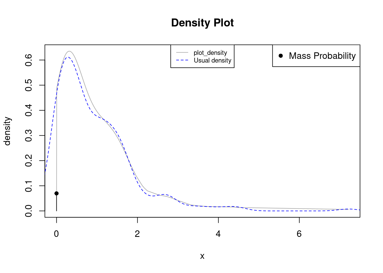
In the previous example the data is non-negative and exhibits repetitions in 0. plot_density detects such repetitions as statistically significant and displays the proportion as a single dot connected with a black line. The density now doesn’t exhibits positive probability in the negative numbers (as opossed to stats::density in blue).
108.4.2 Non-positive data with repetitions
We now center our attention to negative data, e.g. credit due. In such cases density in positive values would be counter intuitive.
set.seed(123)
credit <- c(rep(0, 20), rep(-1, 30), -rgamma(300, 8, 1))
plot_density(credit, bw=0.5)
lines(density(credit), col="blue", lty=2)
legend("topleft", legend=c("plot_density", "Usual density"),
       col=c("darkgray", "blue"), lty=c(1, 2), cex=0.7)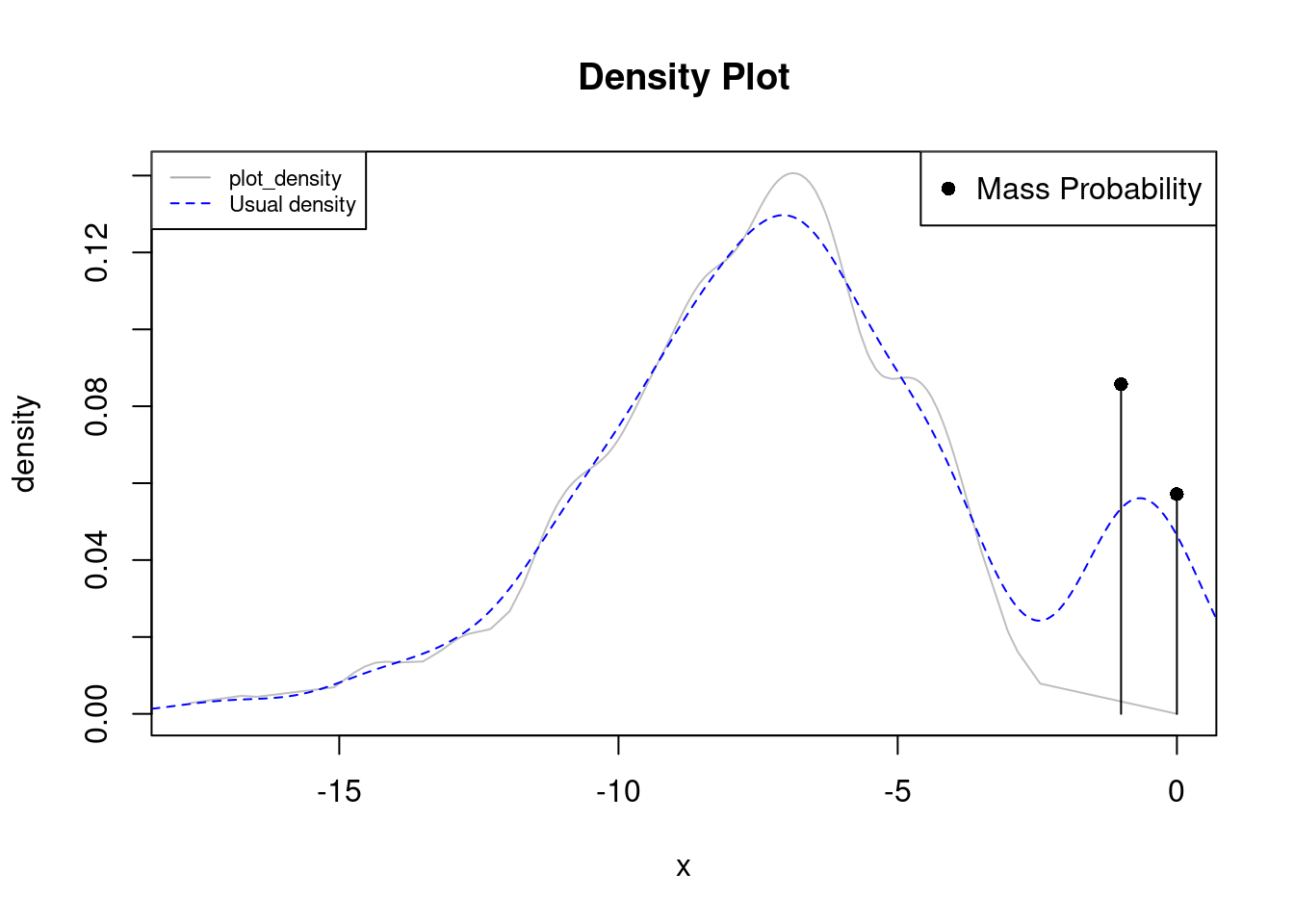
In this case there are two probability mass points at 0 and -1, which may be associated with all the cards with 0 balance, and many having 1 due to, fo example, a cash back promotion for using $1,000 in credit (assume data is in thousands).
plot_density detects such repetitions and excludes them from the other data giving a broader picture of them, the standard density method gives the impression of having a bimodality around -1 when they are actually two repeated values repeated.
108.4.3 Real data with repetitions
We now center in the case of real data that may have repetitions, e.g. mortgage loan amounts in which it is frequent to observe loans in multiples of $1,000.
set.seed(123)
loans <- c(rep(1000, 50), rep(2000, 40), rep(3000, 60), rep(4000, 35), rep(5000, 45), rnorm(500, 3000, 800) )
plot_density(loans, bw=100)
lines(density(loans), col="blue", lty=2)
legend("topleft", legend=c("plot_density", "Usual density"),
       col=c("darkgray", "blue"), lty=c(1, 2), cex=0.7)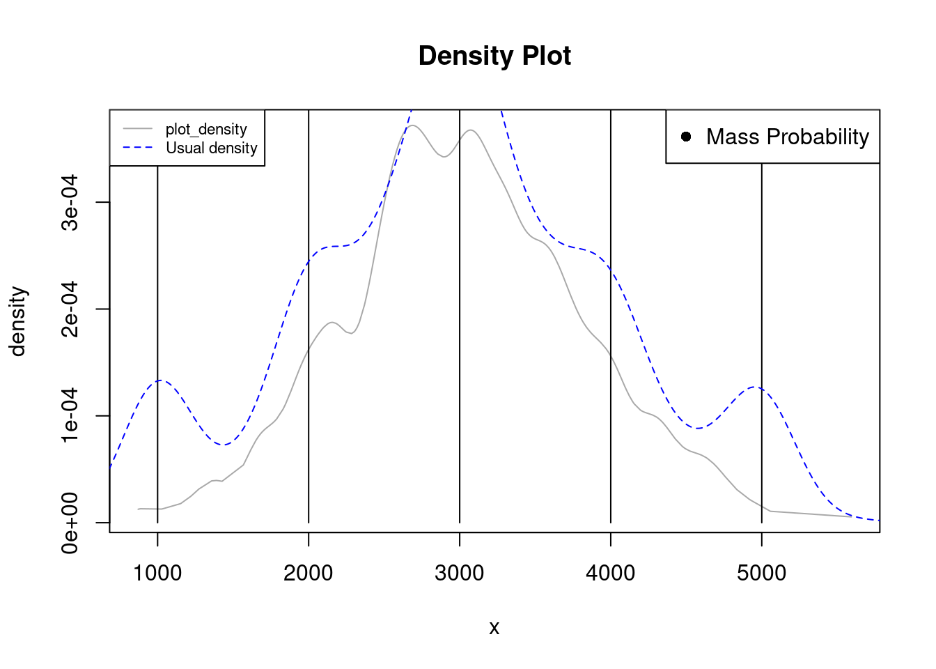
In this case we also had to manually tune the bandwidth by changing the bw parameter. Due to the span of the data, the density is lower than the probability mass, however, the lines are still plotted and they let us know there are repetitions by displaying. This helps to avoid the false impression of many values around the first and last modalities displayed by the blue density.
108.4.4 Real data without repetitions
We finally focus on the general case of real data with no repetitions, in which case plot_density closely resembles stats::density:
set.seed(123)
data <- rt(1000, 3)
plot_density(data)
lines(density(data), col="blue", lty=2)
legend("topright", legend=c("plot_density", "Usual density"),
       col=c("darkgray", "blue"), lty=c(1, 2), cex=0.7)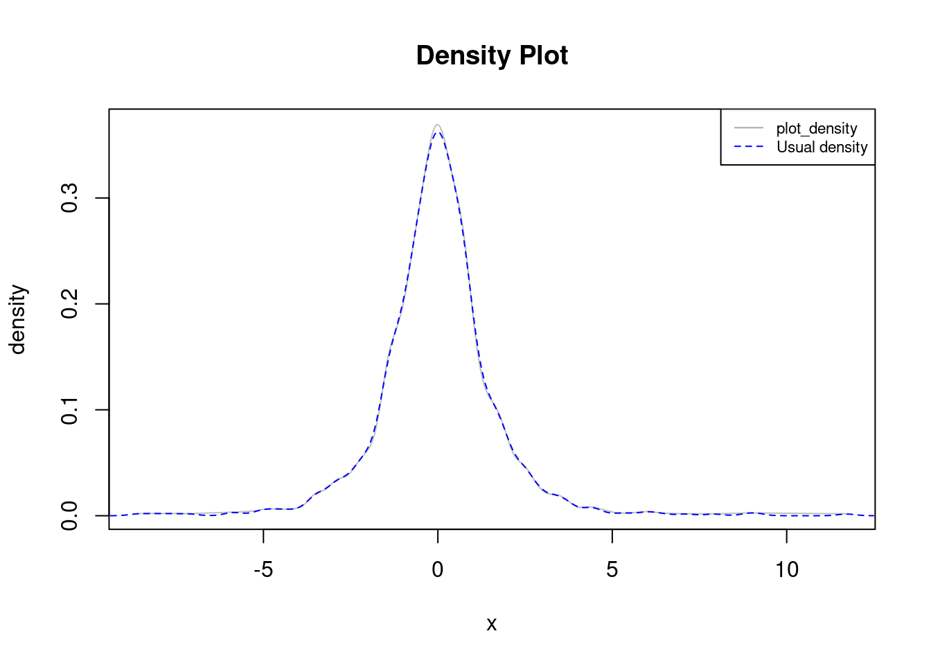
108.5 Conclussion
We introduced a function, plot_density, that can be helpful for univariate visualization in cases with strictly non-negative or non-positive data and in the possible pressence of repetitions.
It generalizes stats::density by using truncated normal kernels for the continuous density, and mixing it with discrete probability mass components if repetitions are found.