69 Introduction to Time Series Analysis in R
Chenqi Wang
69.0.1 Overview
We introduce fundamental time series models including ARMA, GARCH etc. in R and focus on model definitions, process generations and visualizations.
69.0.2 ARMA (Autoregressive-moving-average)
ARMA(p, q): \(y_t=\alpha+\sum_{i = 1}^p\beta_iy_{t-i}+\epsilon_t+\sum_{i=1}^q\theta_i\epsilon_{t-i}\)
where \(y_t\) is the time series, \(\alpha\) is the intercept, \(\beta_i\) and \(\theta_i\) are coefficients, and \(\epsilon_t\) is the white noise.
69.0.2.1 White Noise
\(\epsilon_t\) ~ i.i.d. N(0, \(\sigma^2\)) for some \(\sigma^2>0\).
# generate white noise of length n and s.t.d. b
WN <- function(n, b) {
  x <- rnorm(n, 0, b)
  plot.ts(x, main = paste("white noise of size", n, "and standard deviation", b))
  x
}

e <- WN(500, 1)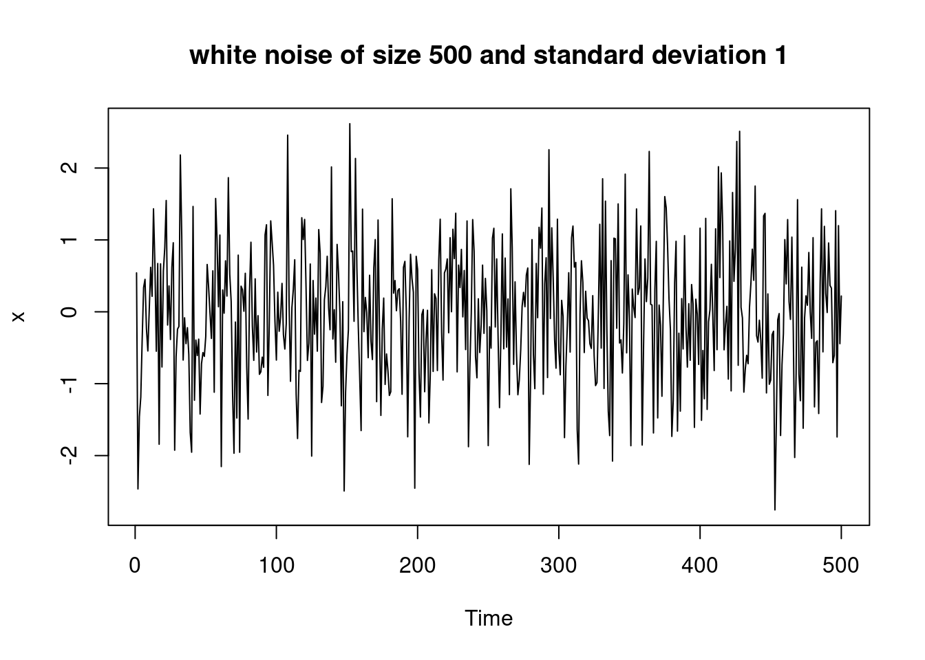
69.0.2.2 AR (Autoregressive)
An ARMA model consists of two parts: AR and MA. Let’s first introduce the AR model:
AR(p): \(y_t=\alpha+\sum_{i = 1}^p\beta_iy_{t-i}+\epsilon_t\)
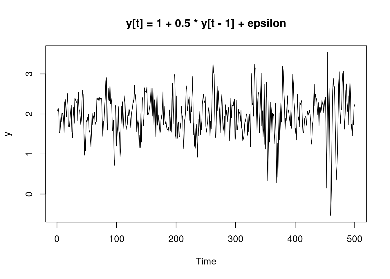
Then we generate an AR(1) model:
# simulation an AR(1) process y_t = b_0 + b_1 * y_{t-1} + epsilon, with data length n
AR1 <- function(b0, b1, b2, n) {
  set.seed(100)
  x <- rnorm(n, 0, b2)
  y <- 0
  y[1] <- b0 / (1 - b1) + x[1]
  for (t in 2 : n) {
    y[t] <- b0 + b1 * y[t - 1] + x[t]
  }

  plot.ts(y, main = paste("y[t] =", b0, "+", b1, "* y[t - 1] + epsilon"))
  y
}

y <- AR1(1, 0.5, 0.2, 500)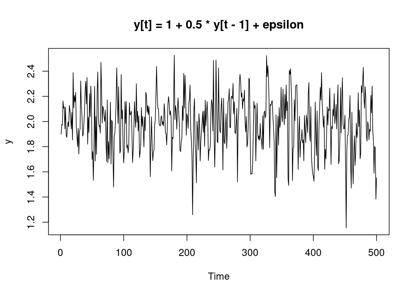
An AR(1) model is weakly stationary if \(|\beta_1|<1\), so our generated model \(y_t=1+0.5y_{t-1}+\epsilon\) is weakly stationary. And we can also see this from the above plot: the mean of the data roughly remains the same, which is what weak stationarity implies.
69.0.2.3 PACF (Partial Autocorrelation Function)
Given a time series \(y_t\) generated by an AR(p) model, to determine the value of p, we can use PACF. The lag-k PACF \(\beta_{kk}\) of a weakly stationary time series measures the contribution of adding the term \(y_{t-k}\) over an AR(k - 1) model, which can be estimated by the Ordinary Least Squares (OLS) estimator \(\hat{\beta_{kk}}\) of the AR(k) model \(y_t=\alpha_{k}+\sum_{i = 1}^k\beta_{ki}y_{t-i}+\epsilon_{kt}\).
pacf(y) 
The above plot indicates that lag \(k\geq 2\) has insignificant contribution, so AR(1) model is enough.
69.0.2.4 ACF (Autocorrelation Function)
lag-k ACf \(\gamma(k):=cov(y_t, y_{t+k})\). Assume the time series \(y_t\) is weakly stationary, then \(cov(y_t, y_{t+k})\) only depends on k.
ACF can also be used to determine the value of p in AR(p) model.
acf(y)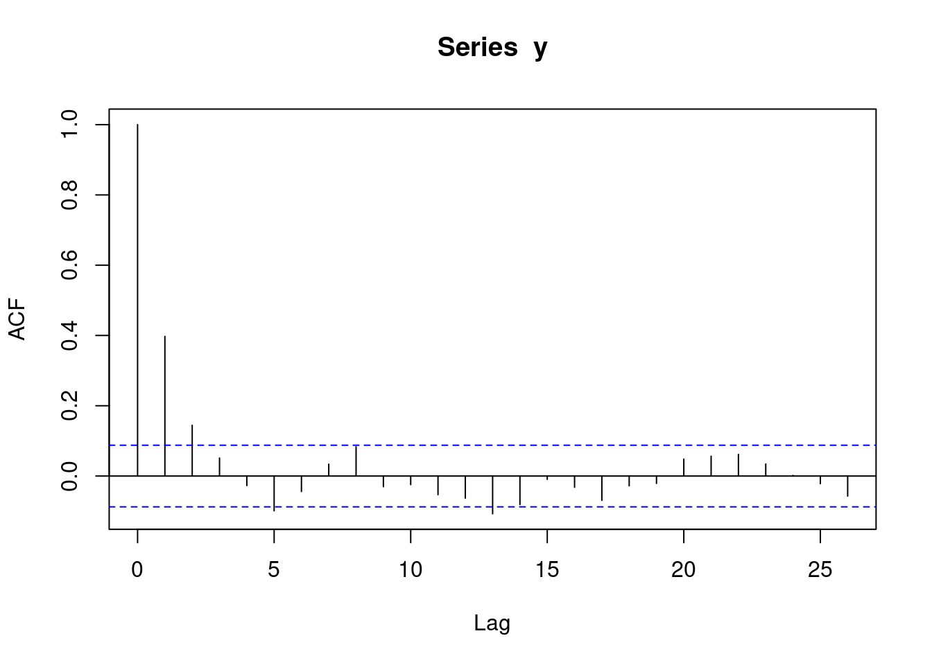
From the above plot we observe that \(y_t\) and \(y_{t+k},k\geq 2\) has insignificant correlation, so again AR(1) is enough.
69.0.2.5 Unit Root Process
A random walk \(y_t=y_{t-1}+\epsilon_t\) is an unit root process, which is not stationary and contains stochastic trend.
# generate the unit root process y[t] = y[t-1] + epsilon
UR <- function(n) {
  set.seed(100)
  x <- rnorm(n, 0, 1)
  y <- 0
  y[1] <- x[1]
  for (t in 2 : n) {
    y[t] <- y[t - 1] + x[t]
  }

  plot.ts(y, main = paste("y[t] = y[t - 1] + epsilon"))
  y
}

y1 <- UR(500)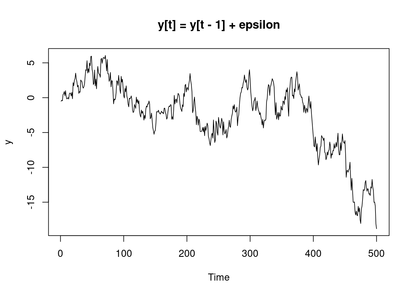
The stochastic trend can be observed in the above plot. Generally the mean of the data goes down, so the time series is not stationary.
69.0.2.6 MA (Moving-average)
MA(q): \(y_t=\alpha+\epsilon_t+\sum_{i=1}^q\theta_i\epsilon_{t-i}\)
Generate a MA(1) model:
# generate MA(1) model y[t] = a + e[t] + r * e[t-1] with data length n
MA1 <- function(a, r, n) {
  set.seed(100)
  e <- rnorm(n, 0, 0.2)
  y <- 0
  y[1] <- a + e[1]
  for (t in 2 : n) {
    y[t] <- a + e[t] + r * e[t - 1]
  }

  plot.ts(y, main = paste("y[t] =", a, "+ e[t] +", r, "* e[t-1]"))
  y
}

y2 <- MA1(1.2, 0.3, 500)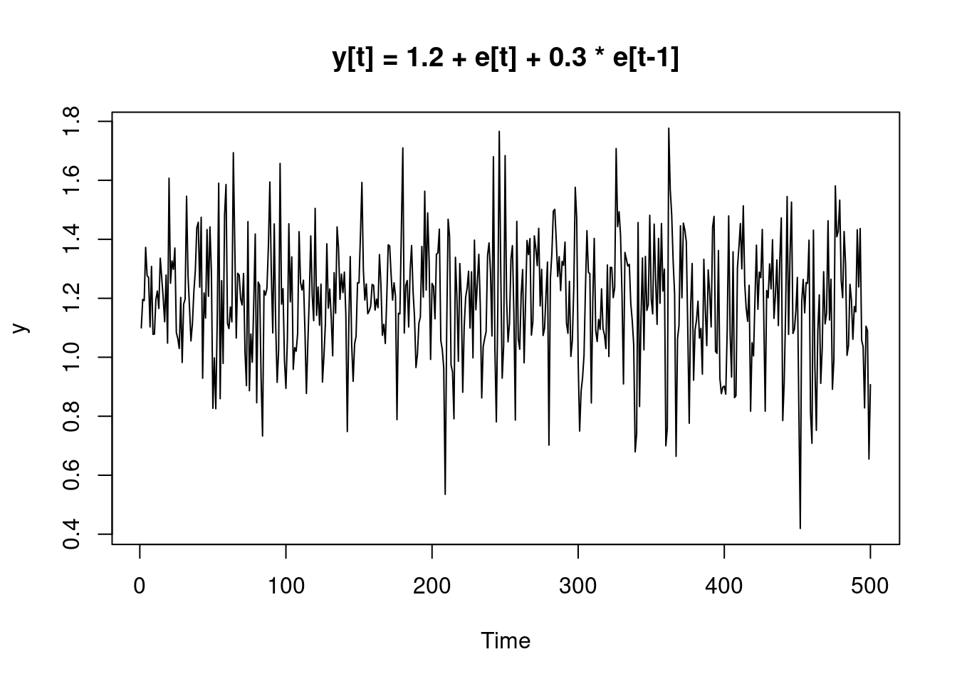
For MA(q) model, \(\forall k>q\) ACF \(\gamma(k)=0\). So it’s easy to ACF to determine q.
acf(y2)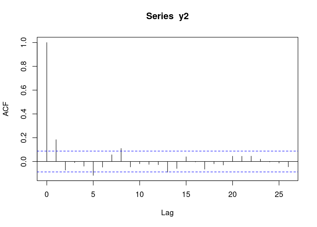
We can observe from the above plot that q should be 1.
69.0.2.7 ARIMA (Autoregressive-integrated-moving-average)
Define the lag operator \(Ly_t:=y_{t-1}\), and \((1-L)^d:=(1-L)[(1-L)^{d-1}]\) (i.e. d order difference). If \((1-L)^{d-1}y_t\) is not weakly stationary but \((1-L)^dy_t\) is weakly stationary for \(d>0\), and \((1-L)^dy_t\) is an ARMA(p, q) process, then \(y_t\) is called an ARIMA(p, d, q) process.
We can use arima() in R to estimate an ARIMA model:
##
## Call:
## arima(x = y2, order = c(0, 0, 1), method = "ML")
##
## Coefficients:
##          ma1  intercept
##       0.2244     1.1903
## s.e.  0.0469     0.0110
##
## sigma^2 estimated as 0.0401:  log likelihood = 94.63,  aic = -183.25
69.0.3 GARCH (Generalized Autoregressive Conditional Heteroskedasticity)
AR(1) - GARCH(s, m):
\(y_t=\phi_0+\phi_{1}y_{t-1}+\epsilon_t\)
\(\epsilon_t = \sigma_t\eta_t\)
\(\sigma_t^2=\alpha_0+\sum_{i=1}^s\beta_i\sigma_{t-i}^2+\sum_{i=1}^m\alpha_i\epsilon_{t-i}^2\)
where \(var(\epsilon_t|y_{t-1})=\sigma^2(y_{t-1})\) (conditional heteroskedasticity)
GARCH models the second moment information of a time series, while ARIMA models only the level of it.
# AR(1) - GARCH(1, 1) y[t] = a0 + a1 * y[t - 1] + v * epsilon, v[t]^2 = b0 + b1 + v[t-1]^2 + b2e^2, data length n
GARCH <- function(a0, a1, b0, b1, b2, n) {
  set.seed(1000)
  n = n + 500
  x <- rnorm(n, 0, 1)
  y = 0
  v = 0
  a = 0
  v[1] = b0 / (1 - b1 - b2)
  a[1] = sqrt(v[1]) * x[1]
  y[1] = a0 / (1 - a1) + a[1]
  for (t in 2 : n) {
    v[t] = b0 + b1 * v[t - 1] + b2 * a[t - 1] ^ 2
    a[t] = sqrt(v[t]) * x[t]
    y[t] = a0 + a1 * y[t - 1] + a[t]
  }
  y = y[-(1:500)]
  v = v[-(1:500)]
  plot.ts(y, main = paste("y[t] =", a0, "+", a1, "* y[t - 1] + epsilon"))
  z = cbind(v, v)
  z
}

y3 <- GARCH(1, 0.5, 0.02, 0.6, 0.3, 500)